This data set collects the maps of small solar system bodies prepared by Phil Stooke of the University of Western Ontario, including those first archived in PDS in 2003, 18 map sheets added in 2011, five map sheets added in 2012, and 44 map sheets added in 2015. The 44 map sheets added in 2015 are marked [NEW]. They include additonal maps on asteroids Ida, Eros, and Itokawa, as well as maps on additional bodies comet 19P/Borrelly 1, comet 103P/Hartley 2, and asteroid 2867 Steins. A total of 270 map sheets are now included, some based on photomosaics from spacecraft images and some based on shaded relief maps prepared from spacecraft images. The information in this browse facility was provided to PDS by Phil Stooke.
A summary of the map projections is available here. There is an index of the maps listing map properties and source missions here.
These maps are in the public domain but should not be used without proper credit being given. The correct citation to use for these maps is "Stooke. P., Stooke Small Bodies Maps V3.0. MULTI-SA-MULTI-6-STOOKEMAPS-V3.0. NASA Planetary Data System, 2015."
The maps included in this set are intended to help with visualization only, and are not suitable for photometric analysis due to very extensive processing. A description of each of the maps follows.
Note: Starting with this version of the map collection (V3.0), the maps of comets and asteroids have been relabelled where necessary for compliance with the IAU guidelines on coordinate systems. In 2003, the IAU Working Group on Cartographic Coordinates and Rotational Elements produced a revised guideline for the coordinate systems of comets and asteroids, having the effect of reversing the longitudes for comets and asteroids with a positive pole north of the ecliptic (Seidelmann et al. 2005). The resulting change affects some of the descriptions and labels of maps for Ida, Gaspra, Mathilde, Eros, Wild 2, and Borrelly. The maps of asteroid Itokawa and comets Hartley 2 and Steins postdate the change in IAU guidelines and are not affected. Planetary satellite maps are not affected.
Seidelmann, P.K., Archinal, B.A., A’Hearn, M.F., Cruiskshank, D.P., Hilton, J.L., Keller, H.U., Oberst, J., Simon, J.L., Stooke, P., Tholen, D.J., Thomas, P.C.: Report on the IAU/IAG working group on cartographic coordinates and rotational elements: 2003. Celest. Mech. Dyn. Astron. 91, 203–215 (2005)
Contents:
Global photomosaics in various projections.
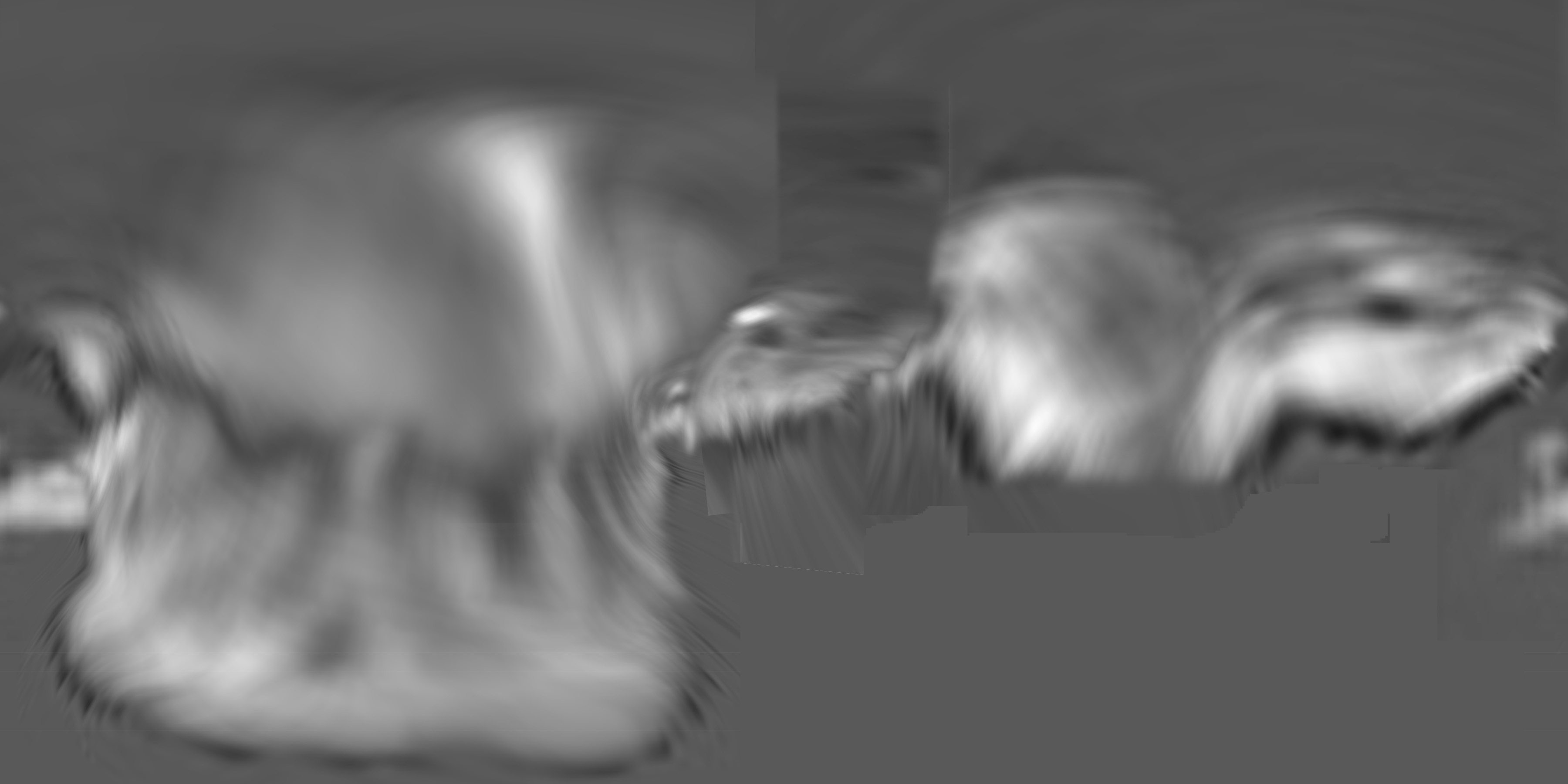
This is an enlarged and improved version of the simple cylindrical mosaic below, which it replaces.
This global photomosaic was constructed by Philip Stooke and Maxim Nyrtsov at the University of Western Ontario. Galileo images were reprojected to simple cylindrical projection based on Peter Thomas's shape model. This version of the map has been superseded by the above mosaic, but is provided for completeness.
Azimuthal Equidistant
Morphographic Equidistant
New Morphograpic Equidistant projections based on a best-fit ellipsoid shape. See the document projections.asc for details.
A. Azimuthal (Morphographic) Equidistant Projection photomosaics.
These cover all of Gaspra in 14 sheets, each 60 degrees by 60 degrees, sheet limits shown on labelled and gridded versions, digital scale 5m/pixel. An additional sheet (sheet 15) covers the whole area imaged at high resolution at 10 m/pixel. Original photomosaic created by P. Stooke, University of Western Ontario, based on positional control by P. Thomas.
Labelled and gridded versions have 5 degree grid spacing. Note: Only sheets
with some high resolution coverage are fully labeled.
B. Globe gores: Composites of the gridded sheets above arranged around the polar sheets in separate northern and southern hemispheres. These may be cut out and assembled to make a globe.
C. Global photomosaics, various projections. The photomosaic data used to create the detailed maps above is also presented in full global form in the following variations:
Morphographic Conformal Projections. As above, but the mosaic is projected
onto the best-fit triaxial ellipsoid to suggest the approximate shape. Only the
northern hemisphere was mapped this way because of the nature of the image
coverage. Six versions are offered: equal area, equidistant, and conformal
(effectively = stereographic) projections of the triaxial ellipsoid, with and
without grids. The grids are not labeled.
| Ungridded | Gridded |
| Equal Area | Equal Area |
| Equidistant | Equidistant |
| Conformal | Conformal |
D. Shaded relief maps.
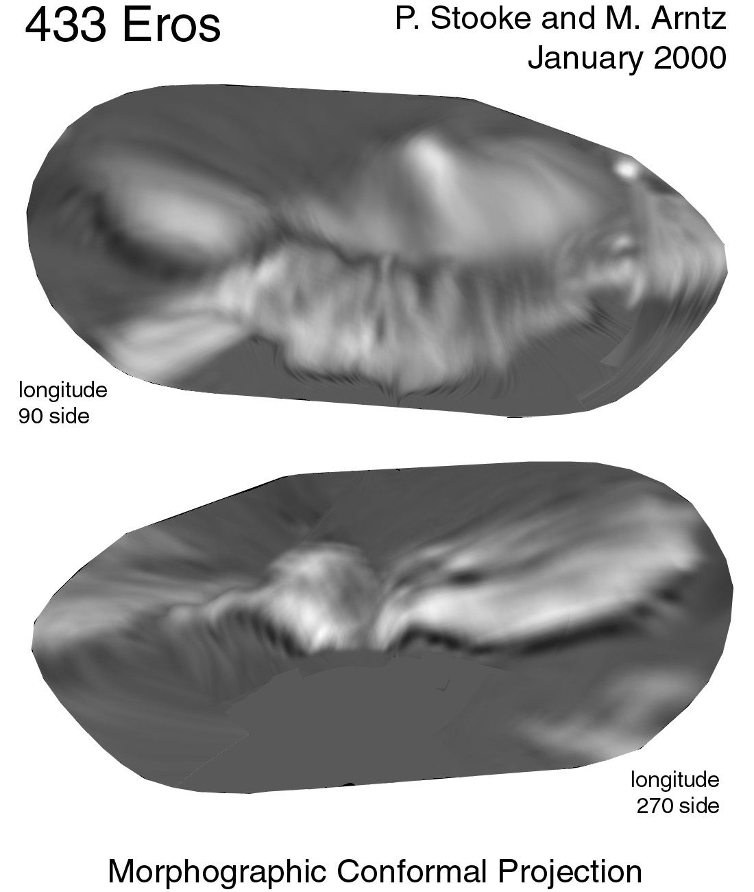
This shaded relief drawing was prepared at lower resolution than the photomosaic and differs slightly in positional control - it is based on earlier work and needs to be redrawn. However, it may still be useful in the absence of any effort by USGS to prepare relief drawings of these worlds. The map is available in several projections. The morphographic conformal projections are shaded relief drawings projected onto the 3D convex hull of the shape, then reprojected to Morphographic Conformal (effectively Stereographic) projection, in two hemispheres centered on the equator and longitudes 90 and 270.
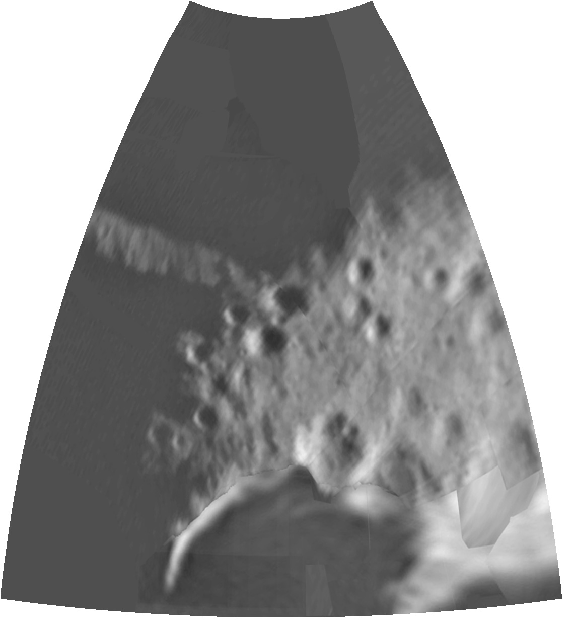
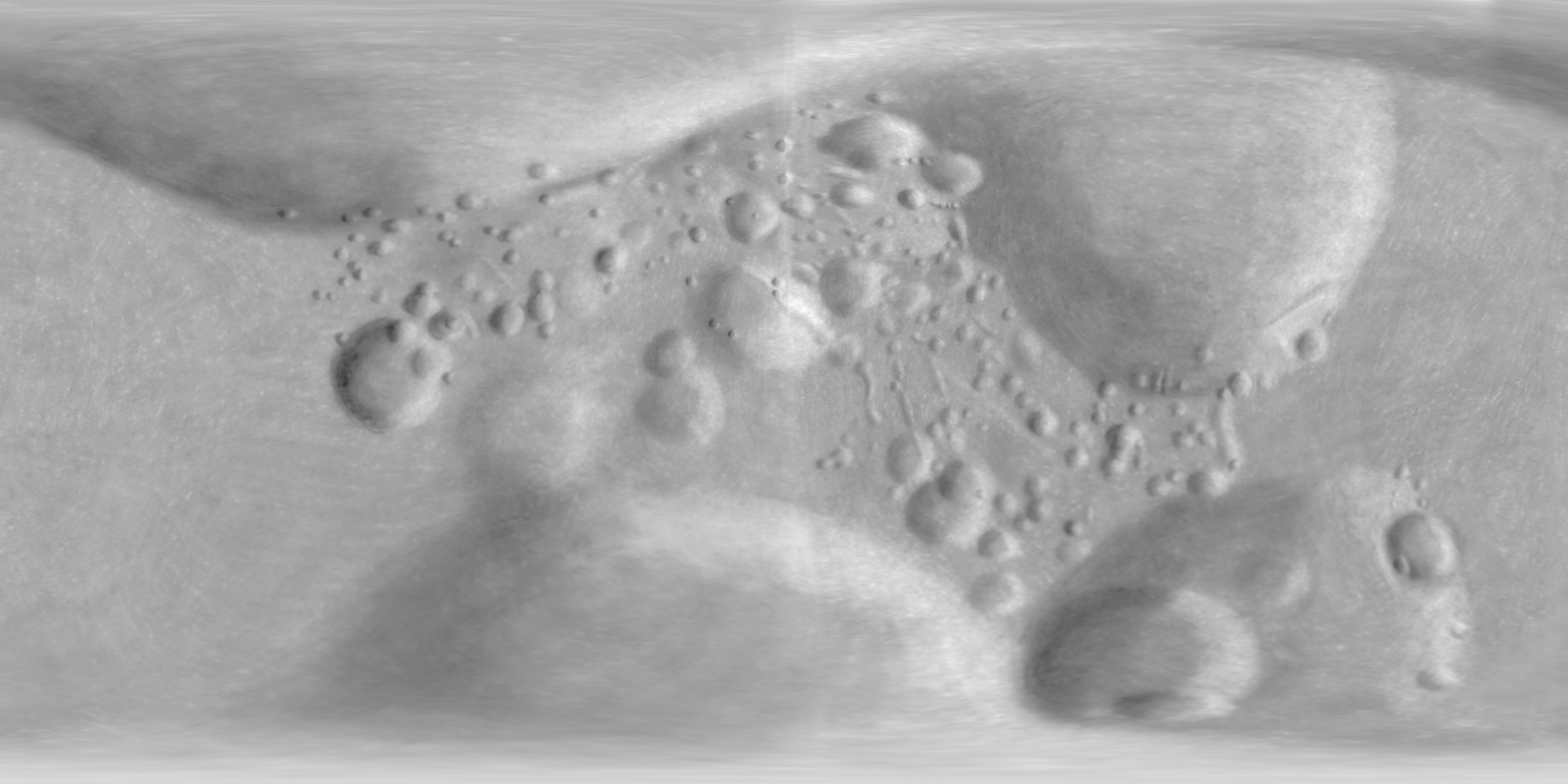
A. Azimuthal (Morphographic) Equidistant Projection photomosaics.
These would cover all of Mathilde in 14 sheets, but limited coverage by the
NEAR camera results in only 4 sheets being produced. Sheet limits are shown on
the gridded and labeled versions. Digital scale is 25 m/pixel. Original
photomosaic created by P. Stooke and J Pfau, University of Western Ontario,
using positional control from P. Thomas. Reference: Thomas, P.C., Veverka, J., Bell, J.F., Clark, B.E., Carcich, B., Joseph, J., Robinson, M., McFadden, L.A., Malin, M.C., Chapman, C.R. and Merline, W., 1999. Mathilde: Size, shape, and geology. Icarus, 140(1), pp.17-27.
| Ungridded | Gridded |
| Sheet 3 | Sheet 3 |
| Sheet 4 | Sheet 4 |
| Sheet 5 | Sheet 5 |
| Sheet 6 | Sheet 6 |
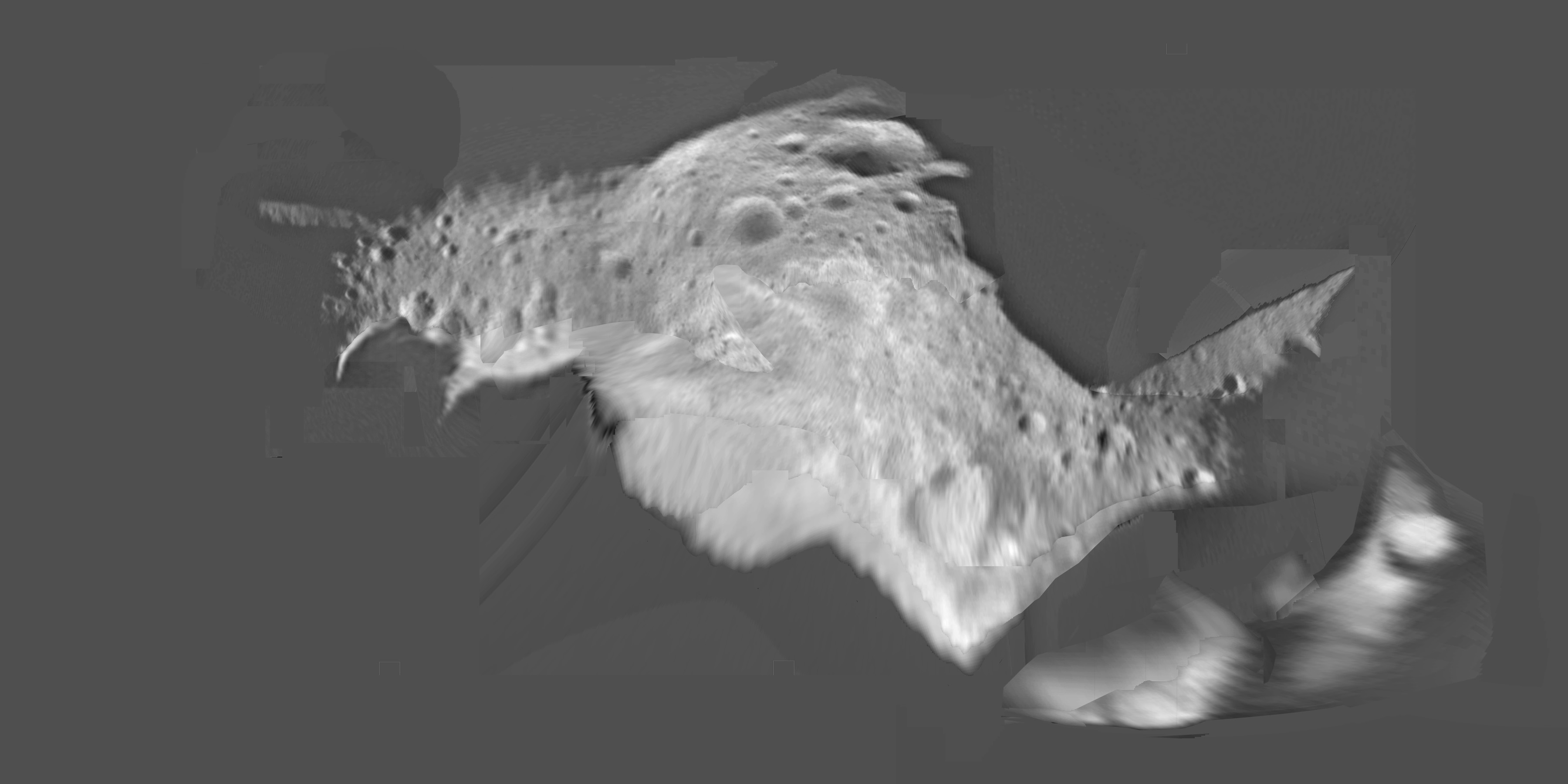
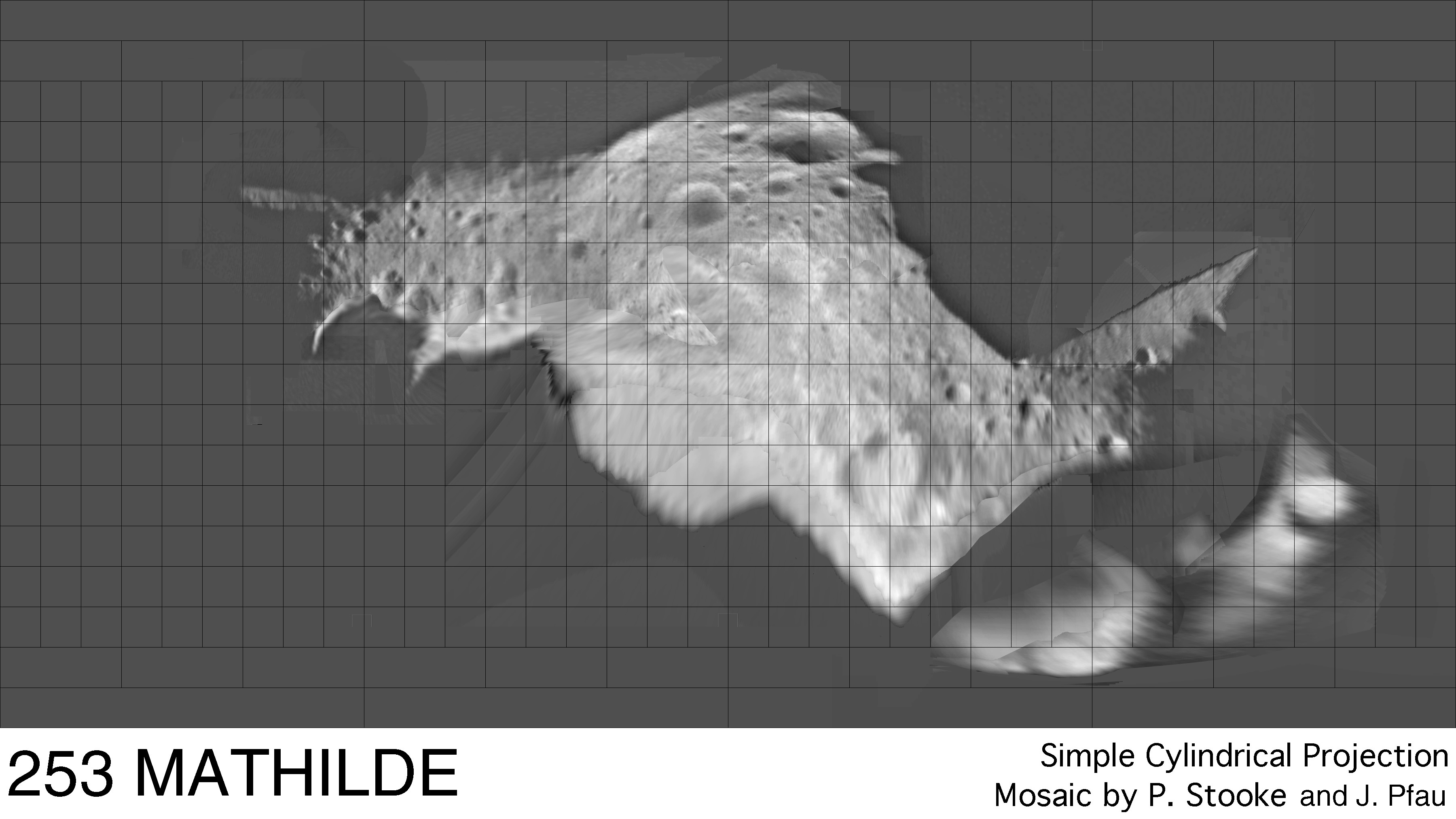
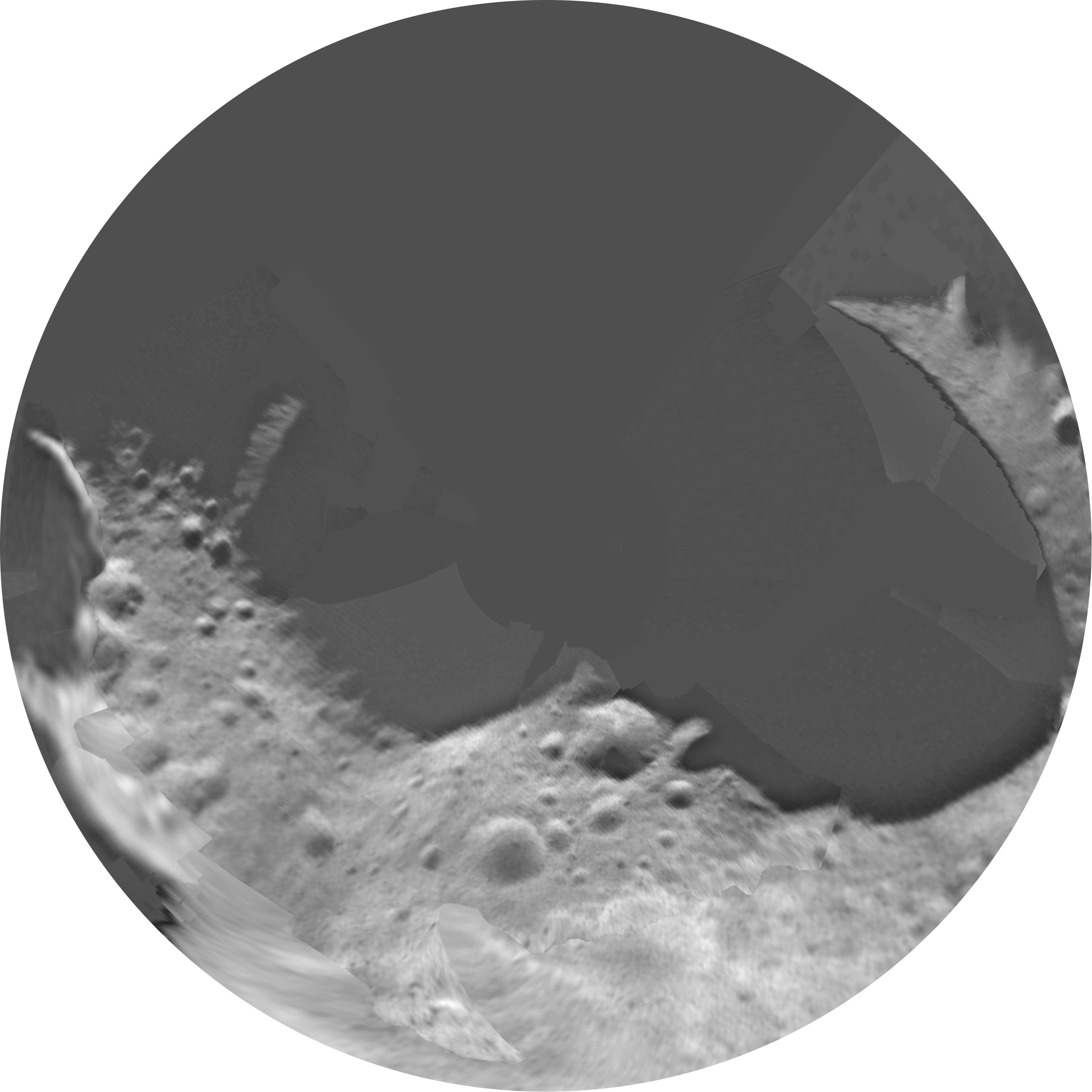
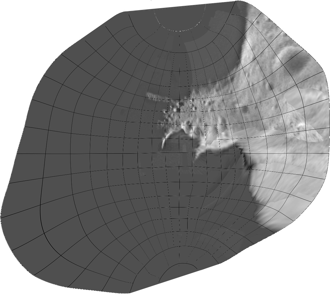
B. Global photomosaics, various projections. The photomosaic data used to create the detailed maps above is also presented in full global form in the following variations.
Morphographic Conformal Projections. As above, but the mosaic is projected
onto the 3D convex hull of the shape model to suggest the approximate shape.
Only the illuminated hemisphere was mapped in this way because of the nature of
the image coverage. Six versions are offered: all are conformal (effectively =
stereographic) projections of the convex hull, but centered on the equator at
longitudes 90, 180, and 270 degrees, with and without grids. The grids are not
labelled, but may be compared with the gridded quadrangle sheets above.
| Ungridded | Gridded |
| Longitude 270 | Longitude 270 |
| Longitude 180 | Longitude 180 |
| Longitude 90 | Longitude 90 |
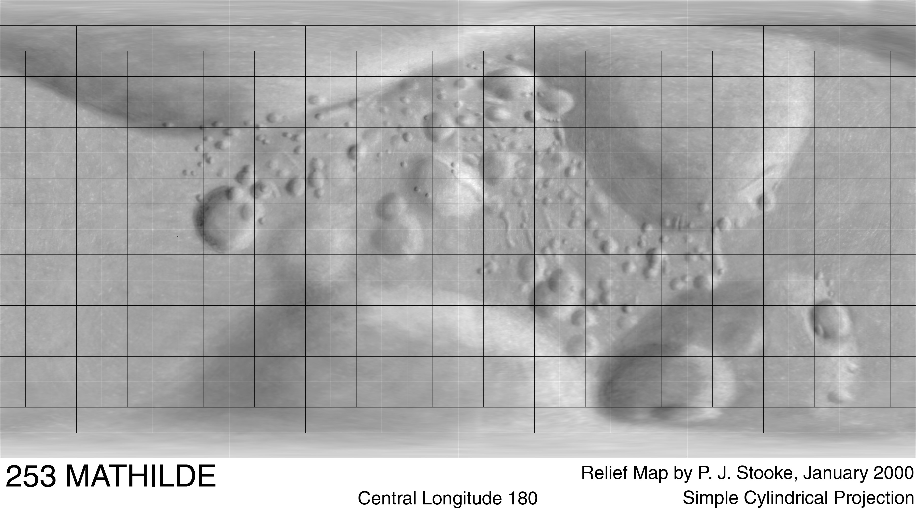
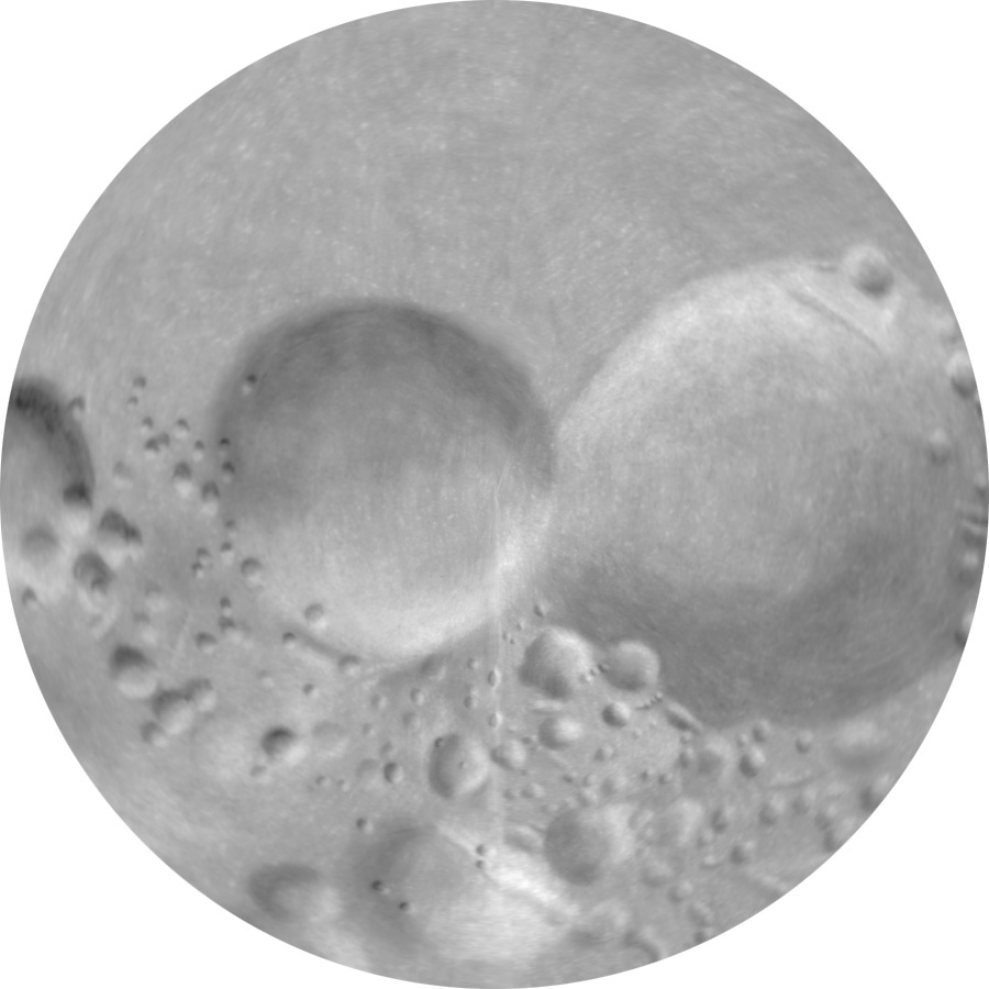
C. Shaded relief maps. This shaded relief drawing by P. Stooke is available in several projections:
(Morphographic conformal projection is the relief drawing projected onto the 3D convex hull of the shape, then reprojected to morphgraphic conformal (effectively stereographic) projection, in three hemispheres centered on the equator and longitudes 90, 180, and 270 degrees.
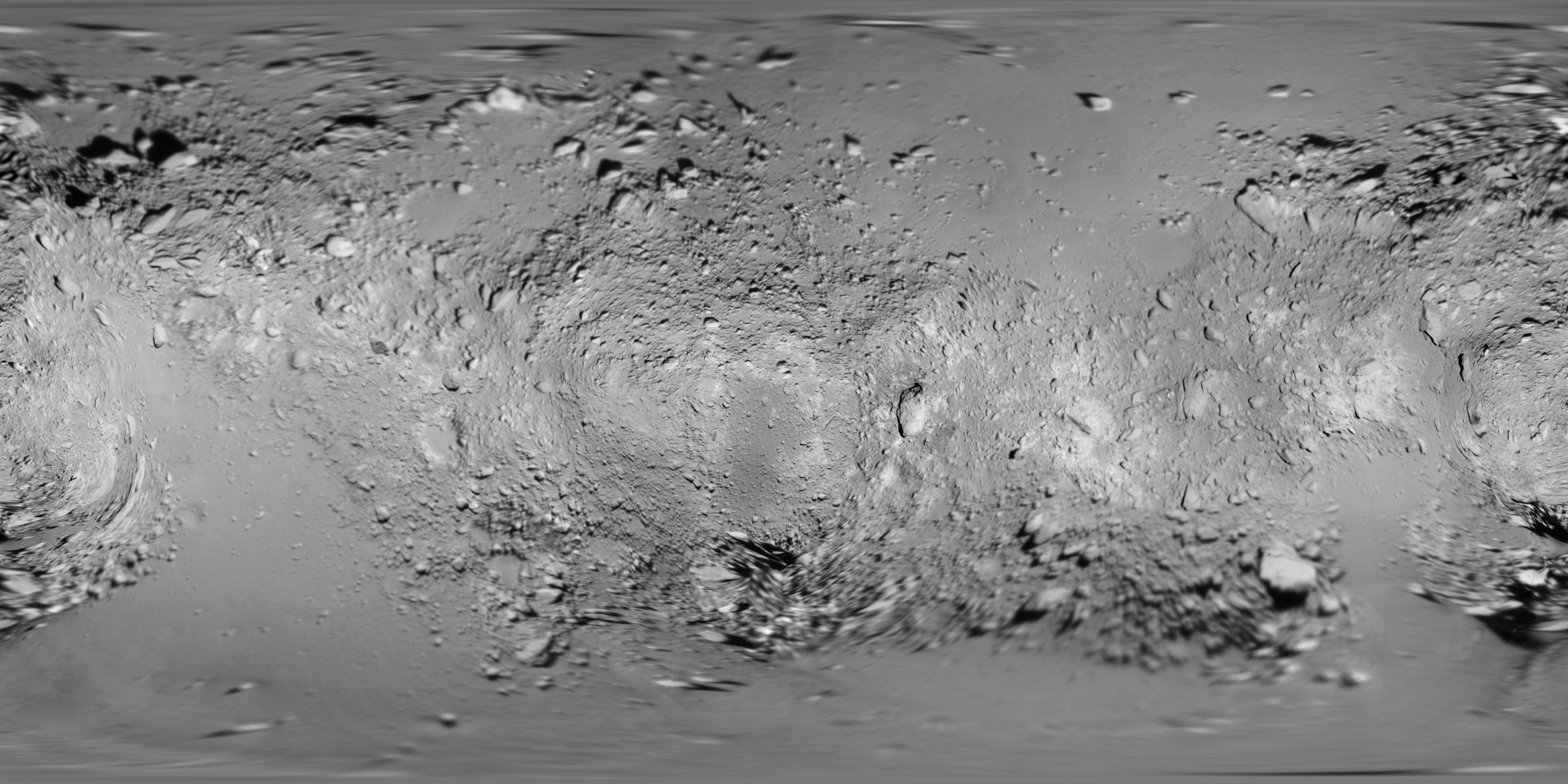
A. Map from NEAR Eros orbital images
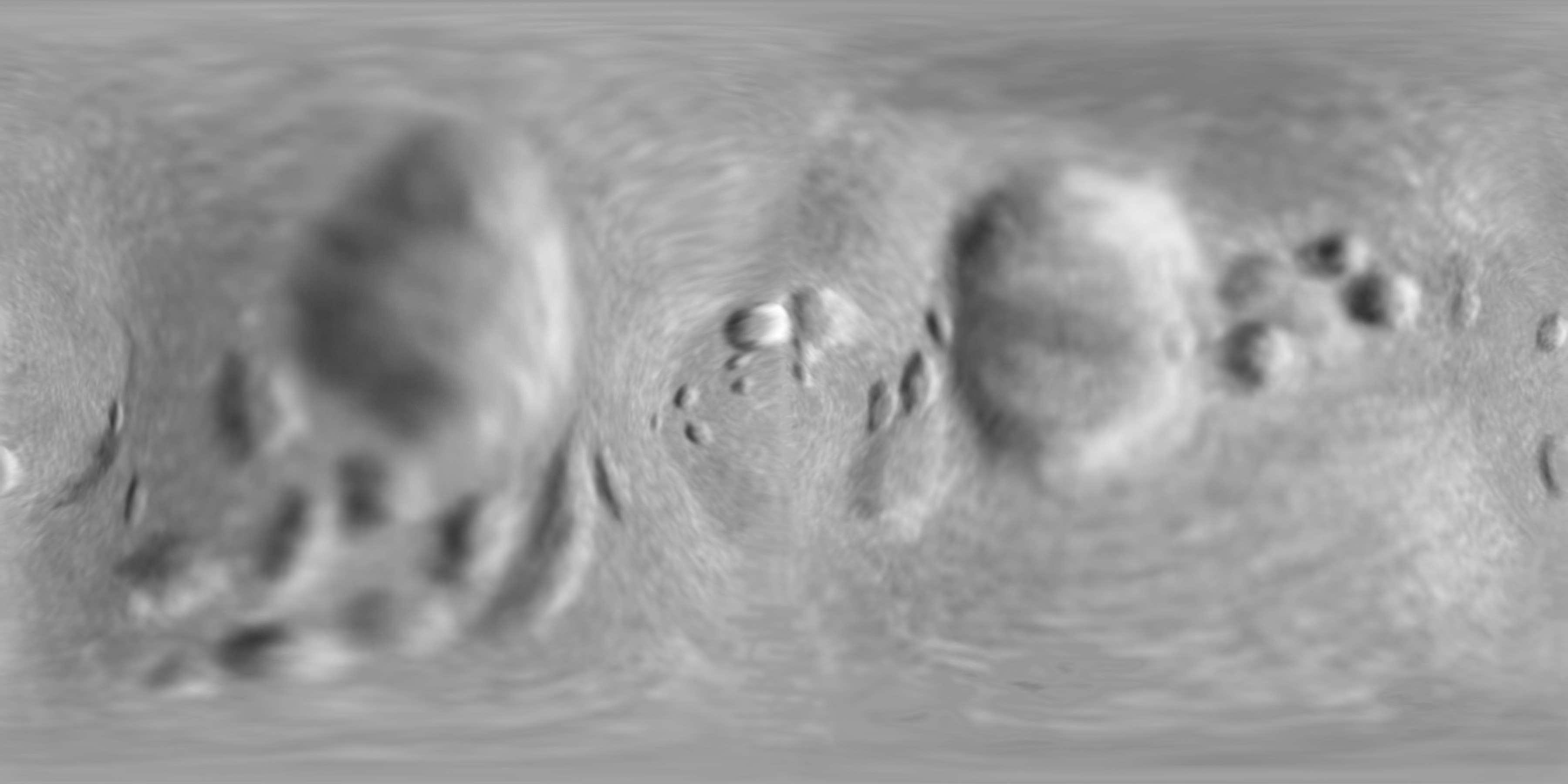
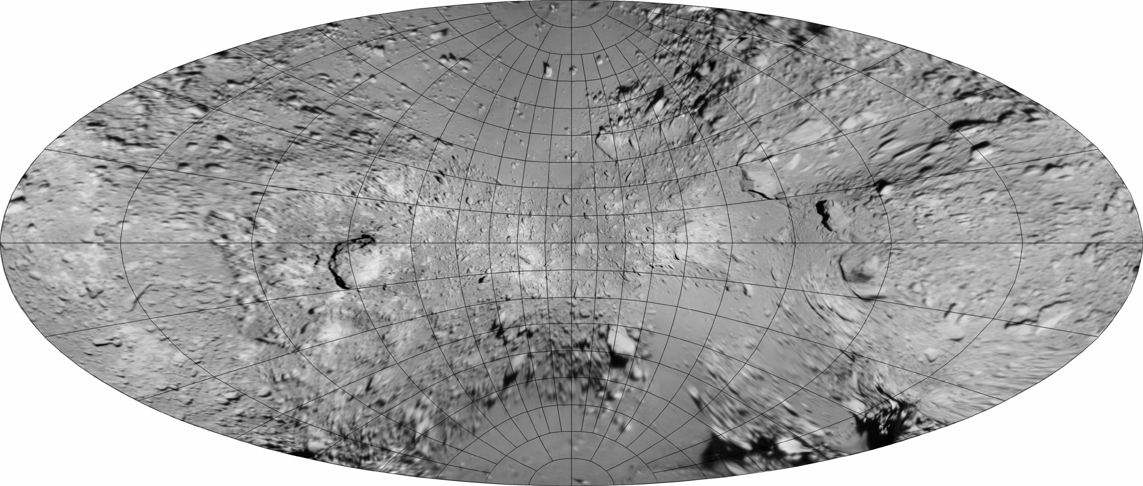
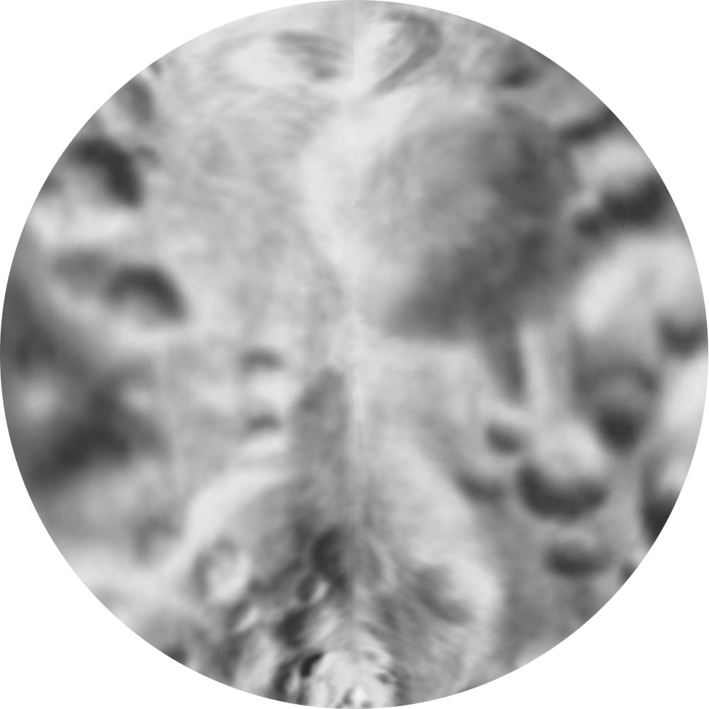
This map is a high resolution photomosaic of 433 Eros. (It is augmented by the reprojected versions provided in section B below.) Control is based on the mosaic produced by the NEAR team and archived in the PDS as NEAR-A-MSI-5-DIM-EROS/ORBIT-V1.0:F4_16_00N000.IMG, but during compilation many errors such as mis-matched mosaic seams in the old mosaic were corrected. In almost every part of the map images were selected with illumination from east to west (sometimes from northeast or southeast). Only in very limited areas, especially near the poles, was it necessary to use images with incompatible lighting. Distortions caused by the irregular shape of Eros are especially apparent near the equator at 310 and 200 longitudes. The resolution and seamless appearance of this mosaic should allow greatly improved visualizations of Eros compared with previous mosaics.
Simple Cylindrical Projection, north at the top, 0 longitude at the left and right edges, 180 degrees at the center, 14400 by 7200 pixels. (40 pixels/degree)
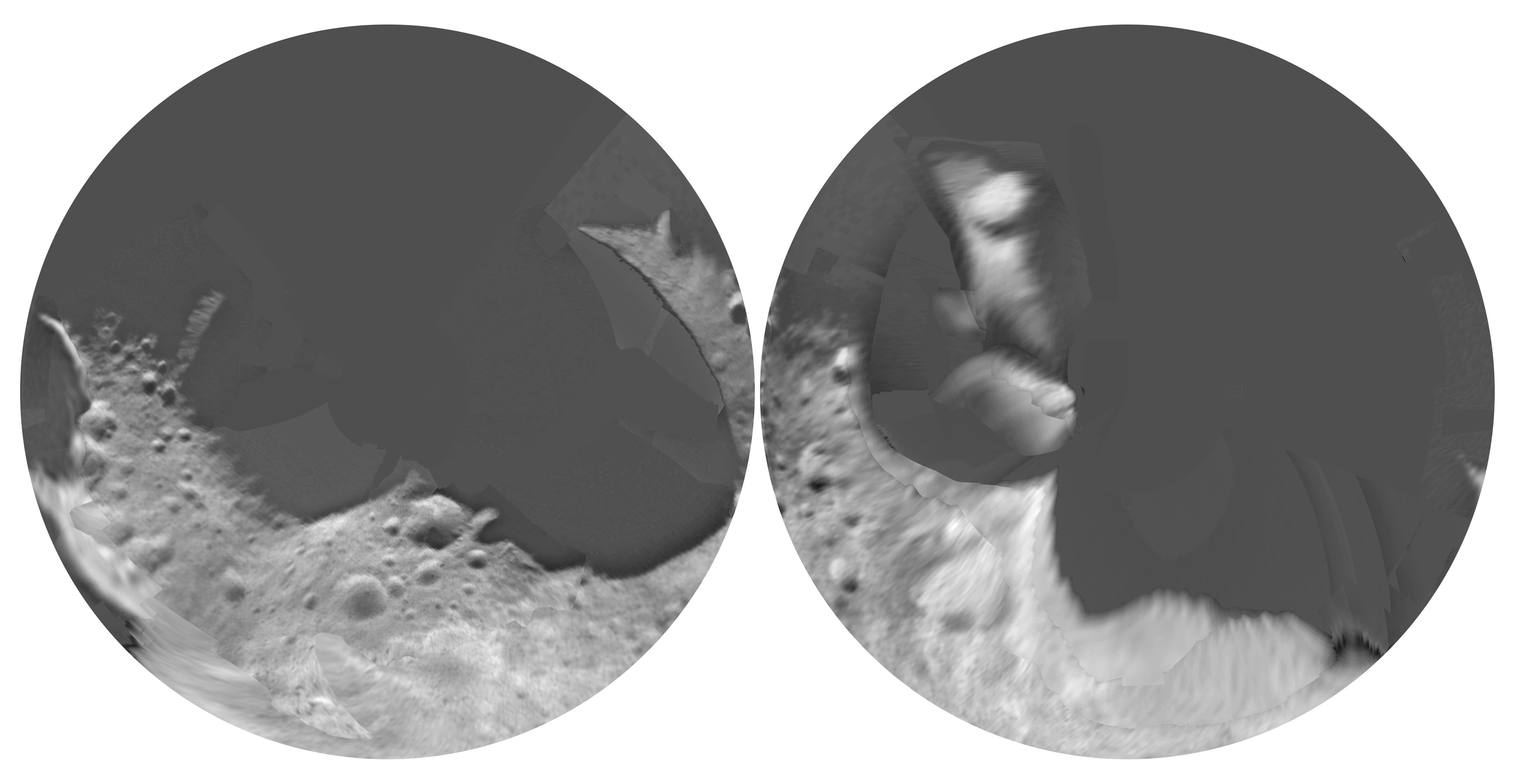
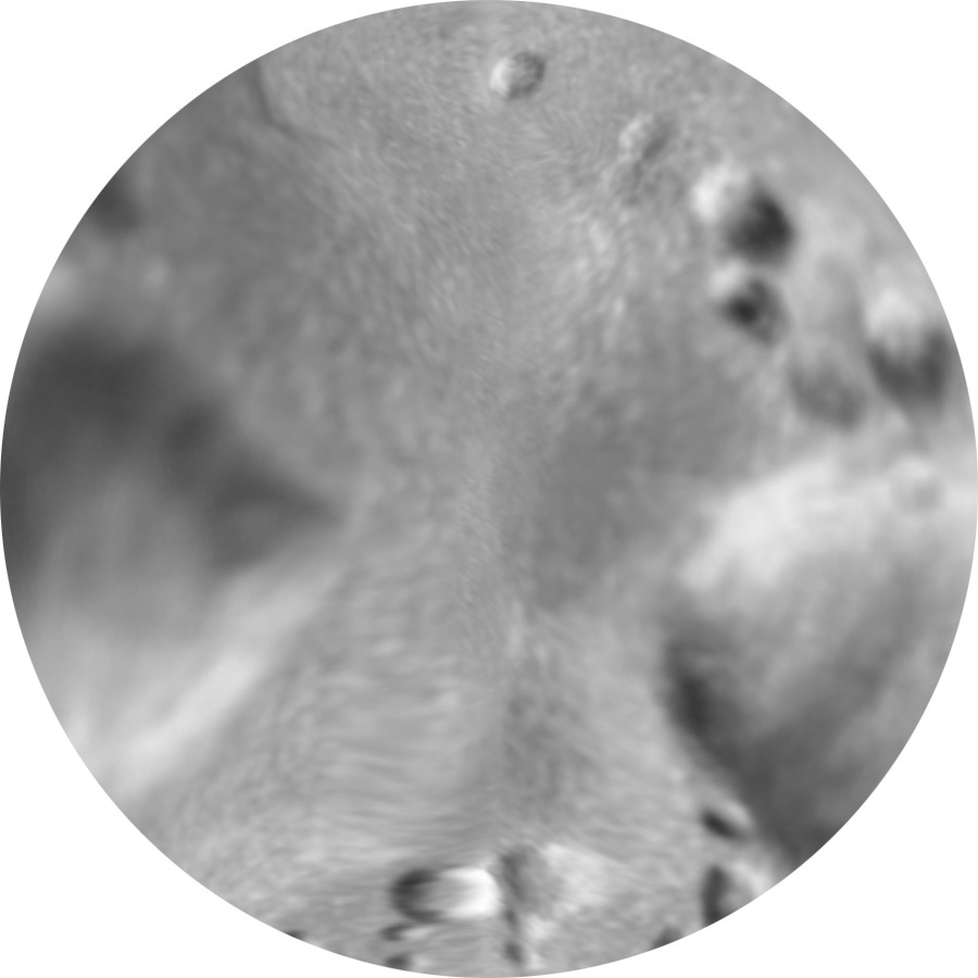
Polar Equidistant Projection North, (latitudes equally spaced), 0 longitude at the top, north pole at center, 50 degrees north at the outer edge.
Polar Equidistant Projection South, (latitudes equally spaced), 0 longitude at the top, south pole at center, 50 degrees south at the outer edge.
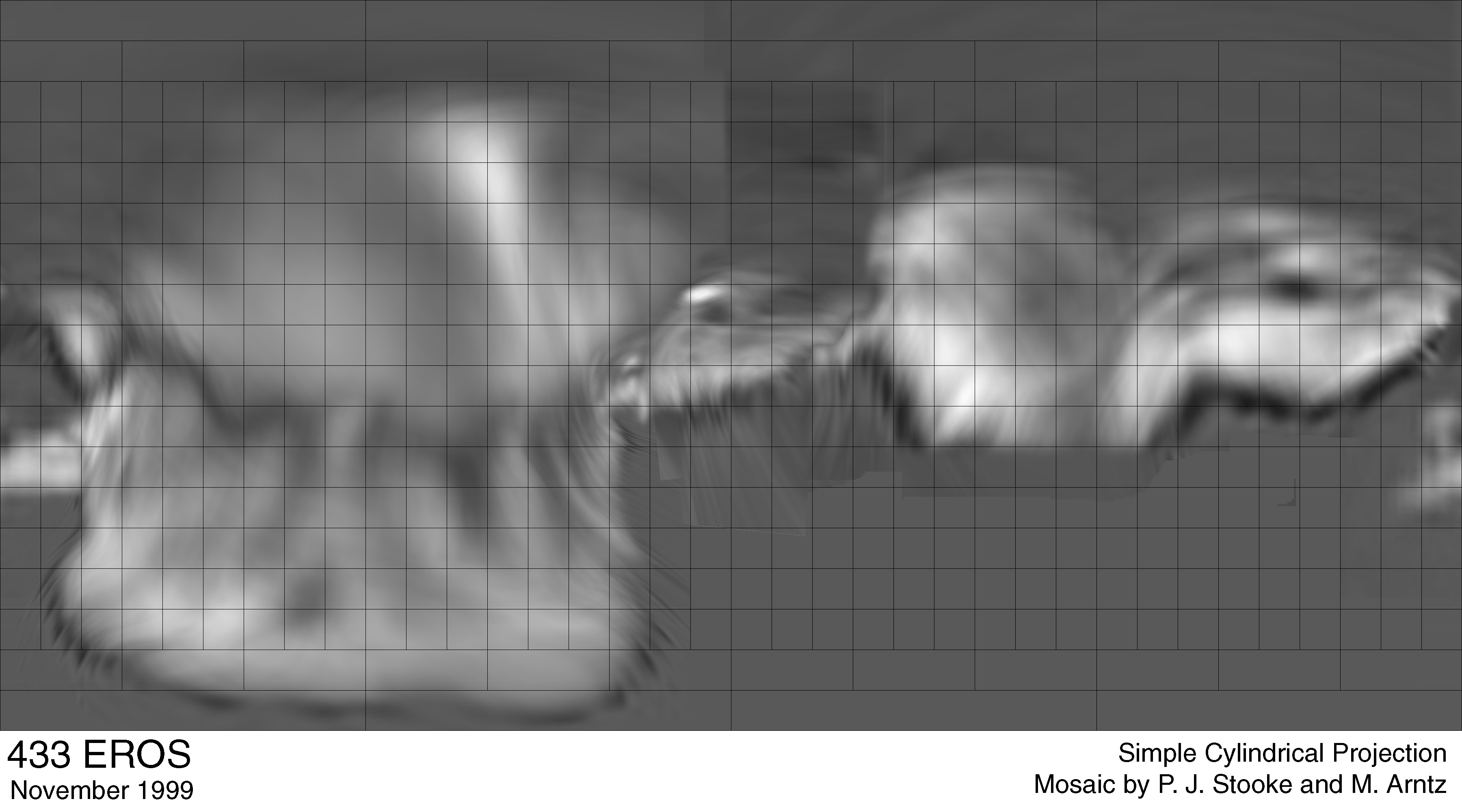
The large cylindrical map (at 20 pixels/degree), colorized, divided into three sections and overlaid with a labelled grid, plus a file containing the two polar areas with grids:
References:
Robinson, M.S. et al., NEAR MSI DIM Eros Global Basemaps V1.0, NEAR-A-MSI-5-DIM-EROS/ORBIT-V1.0, NASA Planetary Data System, 2001. (Available online)
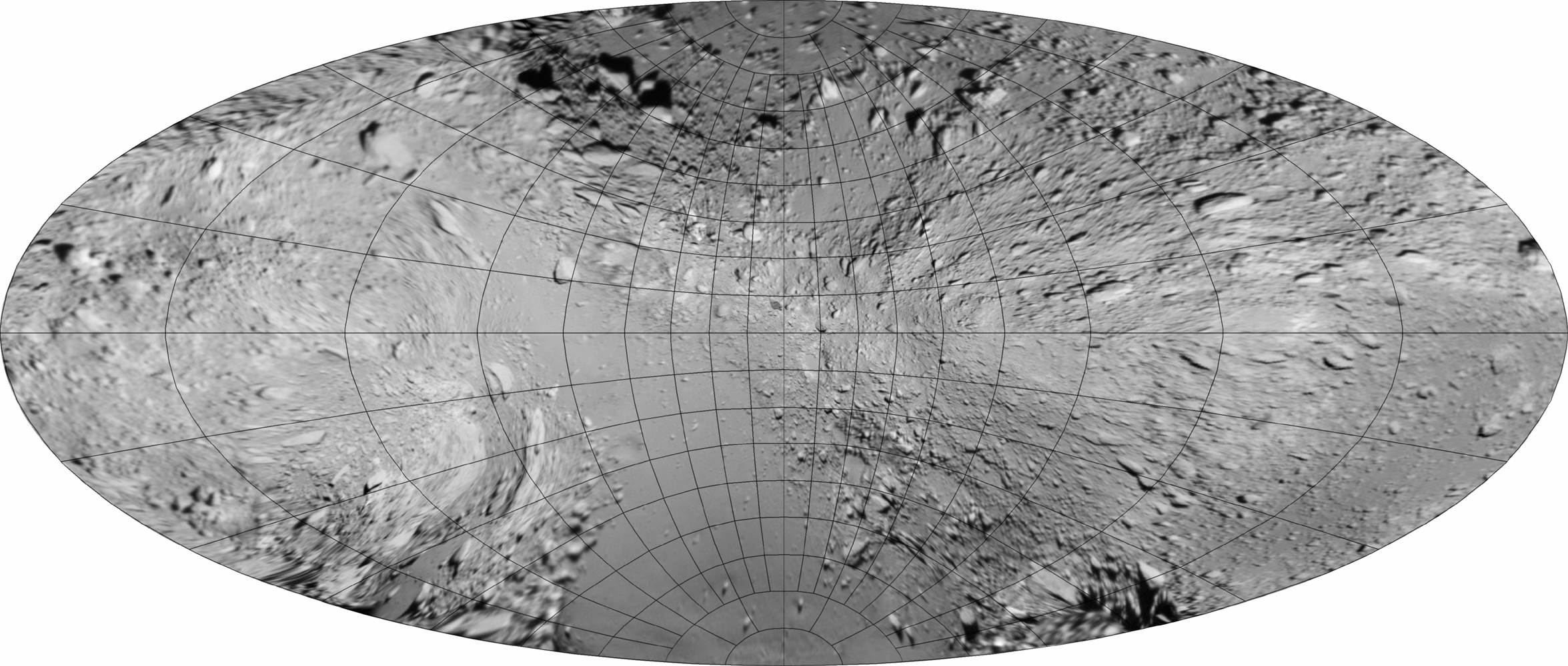
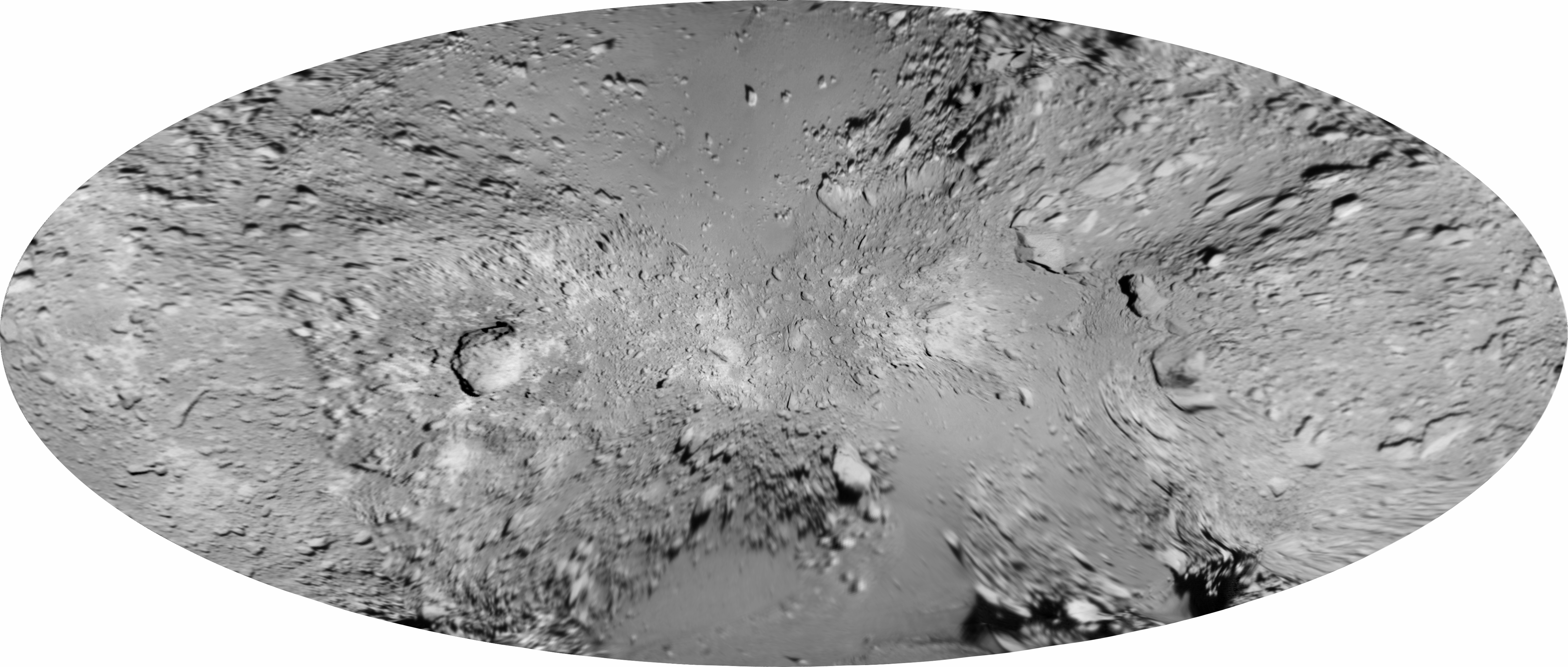
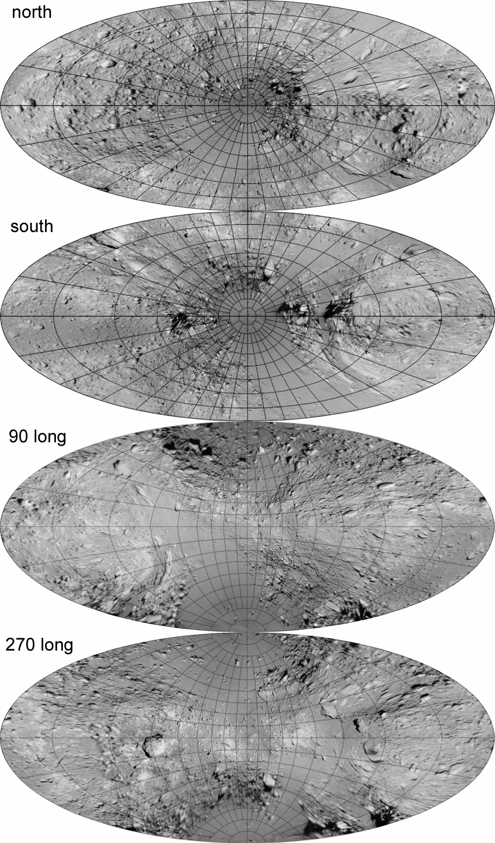
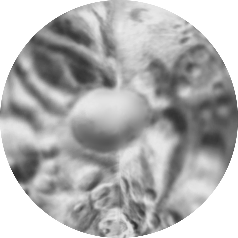
B. Reprojected map from NEAR Eros orbital images
These are reprojected versions of the large cylindrical projection map provided in A above. The purpose is to provide a new form of visualization of the asteroid, as a base for new maps of geological features or other data. Gridded and ungridded versions are provided. A few areas appear more distorted than others, where the true shape of Eros differs most significantly from the ellipsoid.
C. Maps prepared from the NEAR flyby images. They are probably of
historical value only.
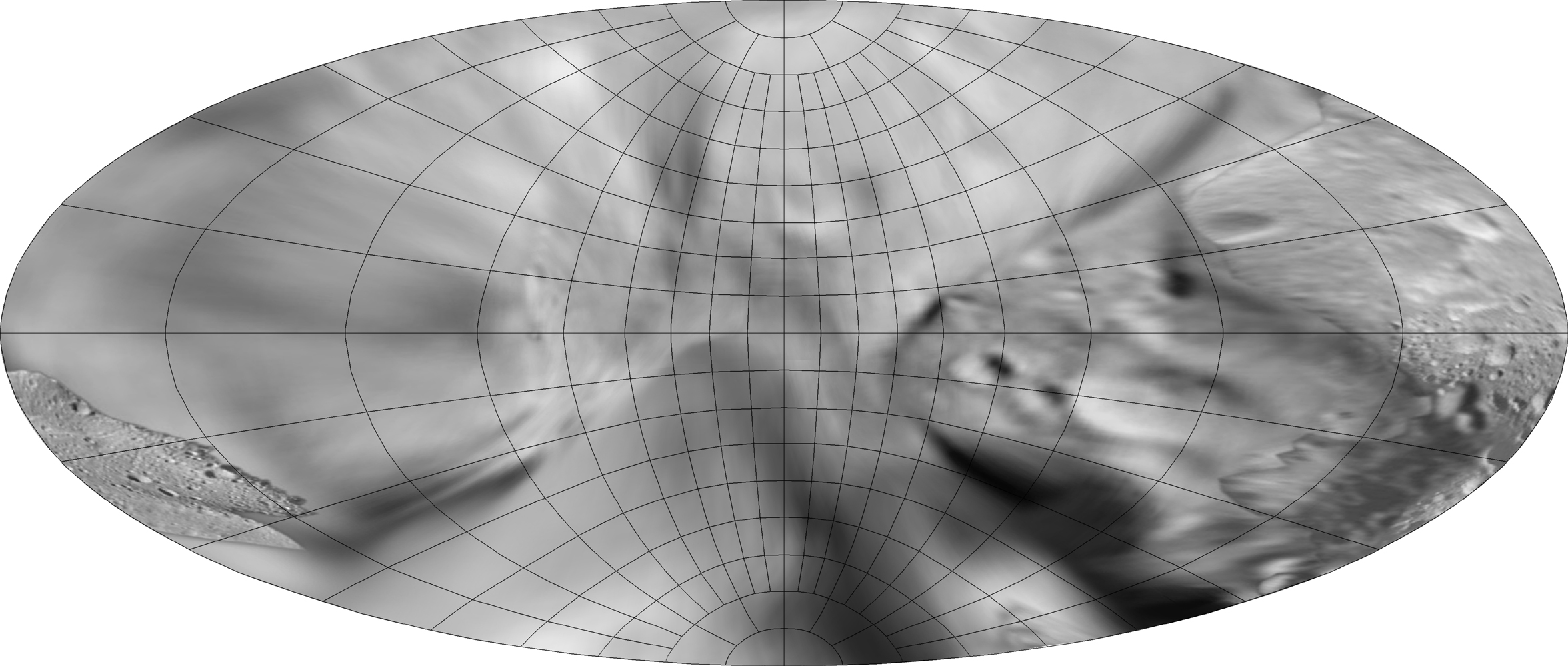
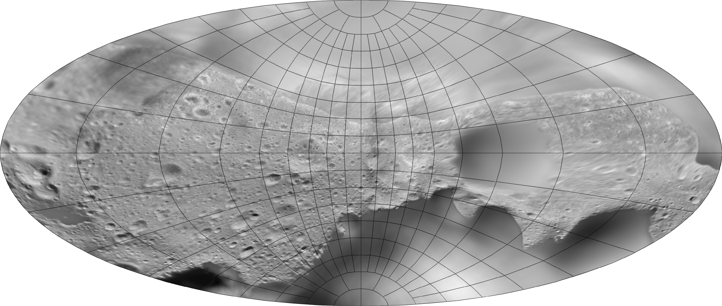
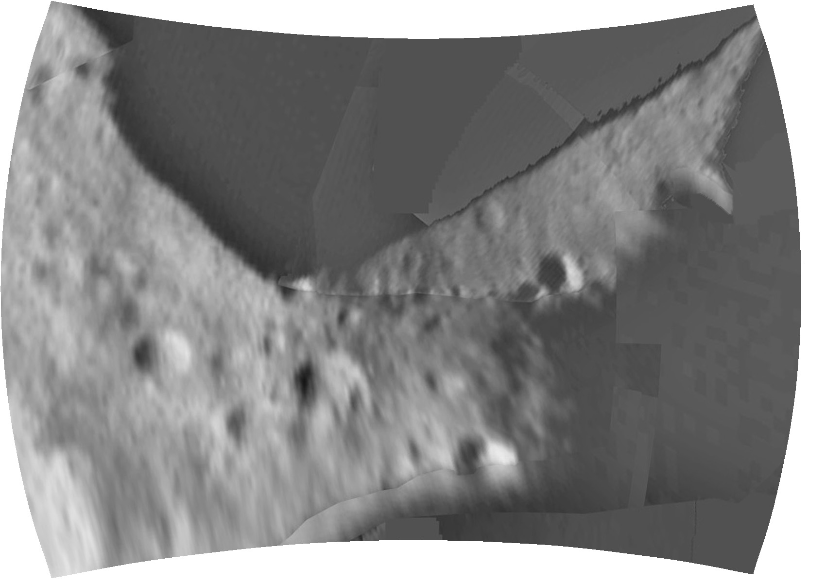
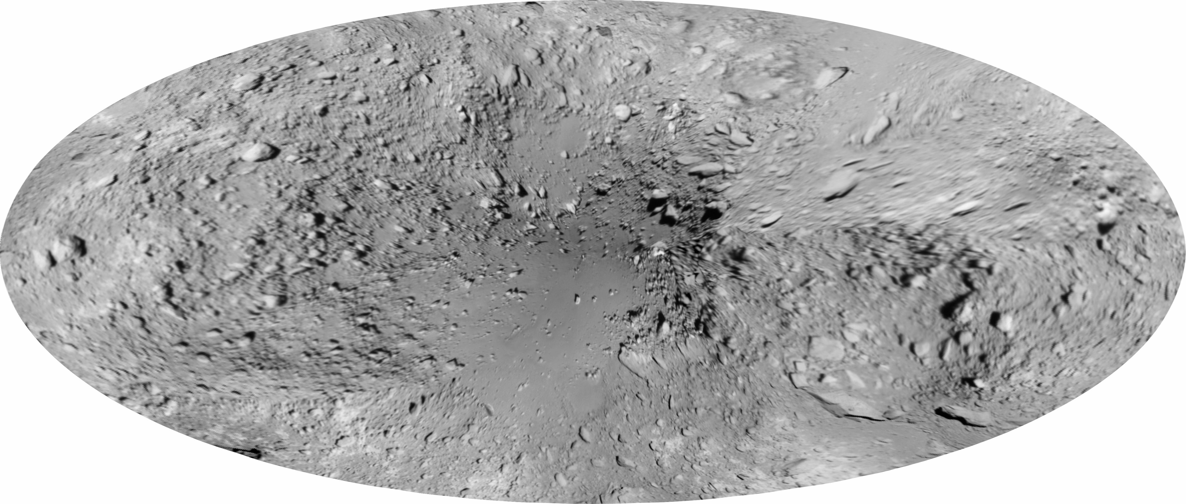
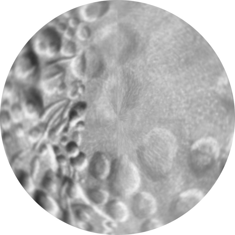
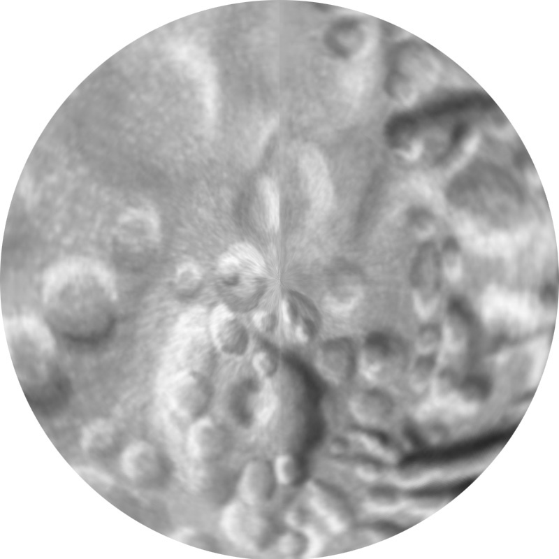
These maps are derived from the topographic model by Gaskell, archived in PDS as HAY-A-AMICA-5-ITOKAWASHAPE-V1.0. The same images with a latitude-longitude grid superimposed were published by Hirata et al. (2009).
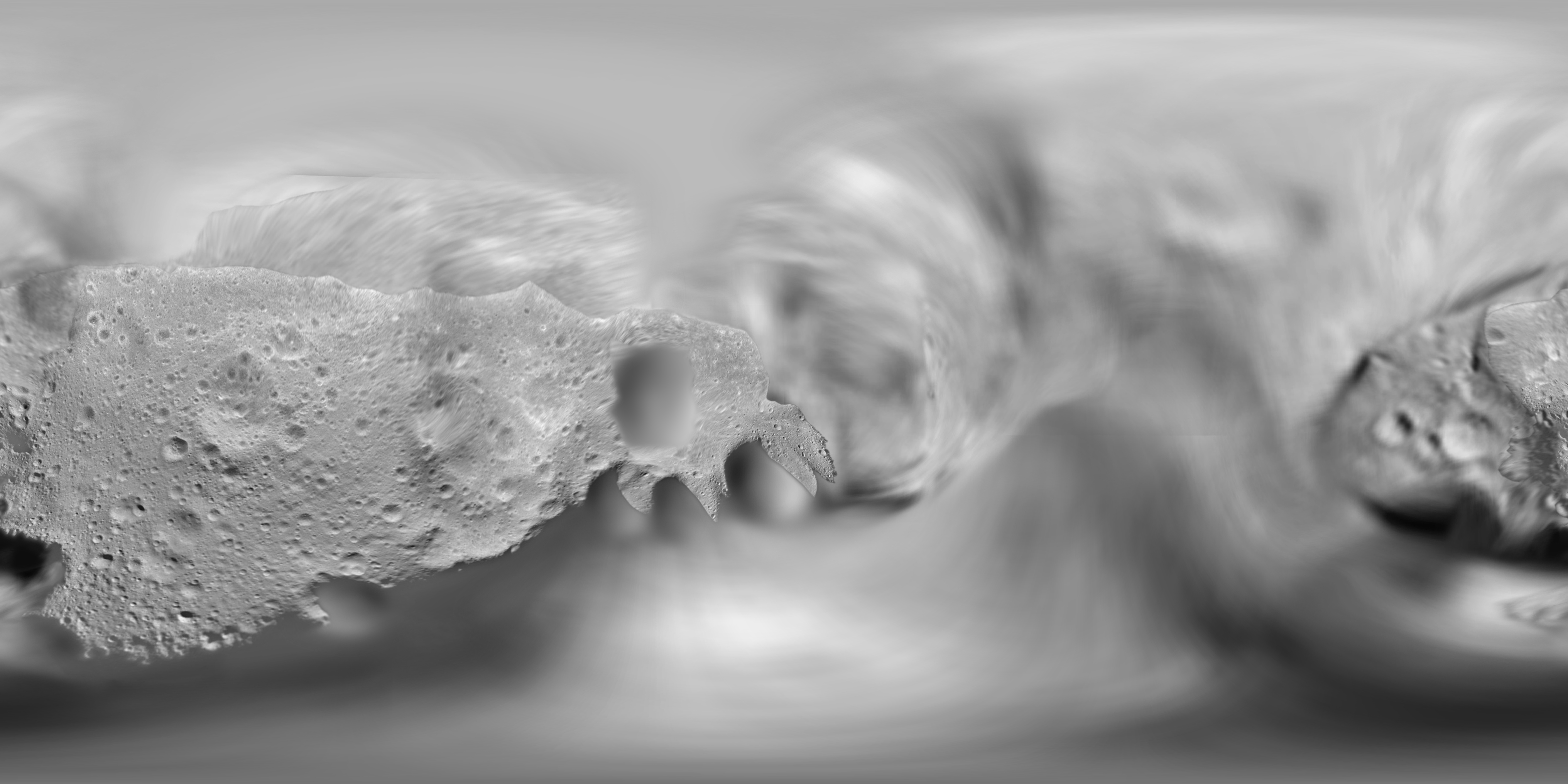
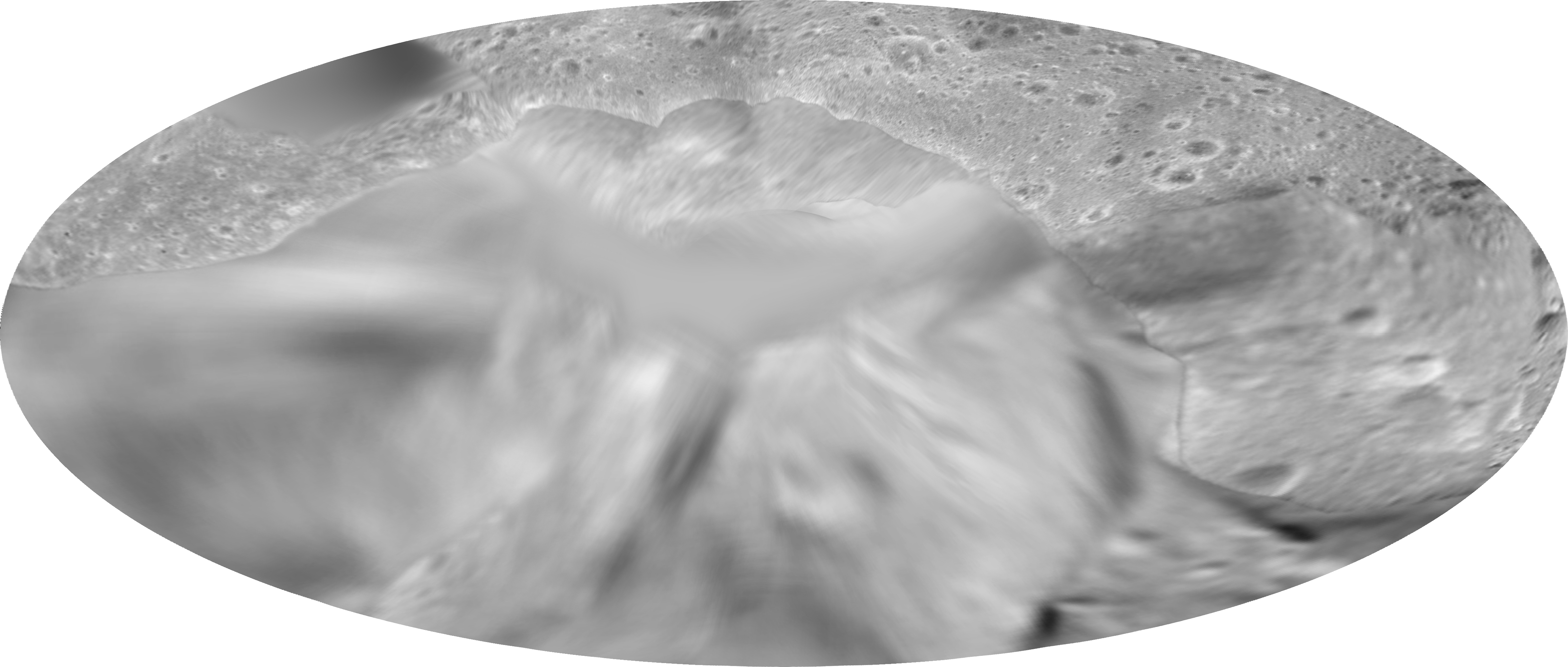
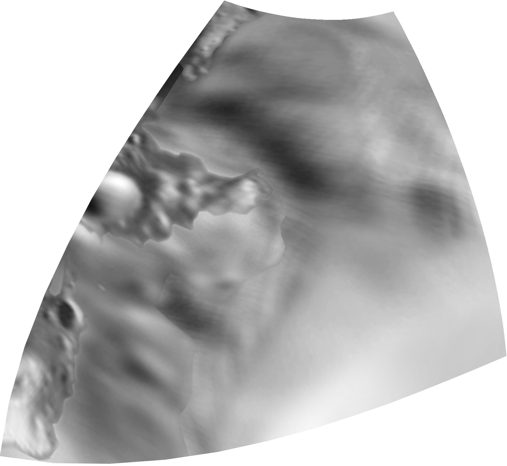
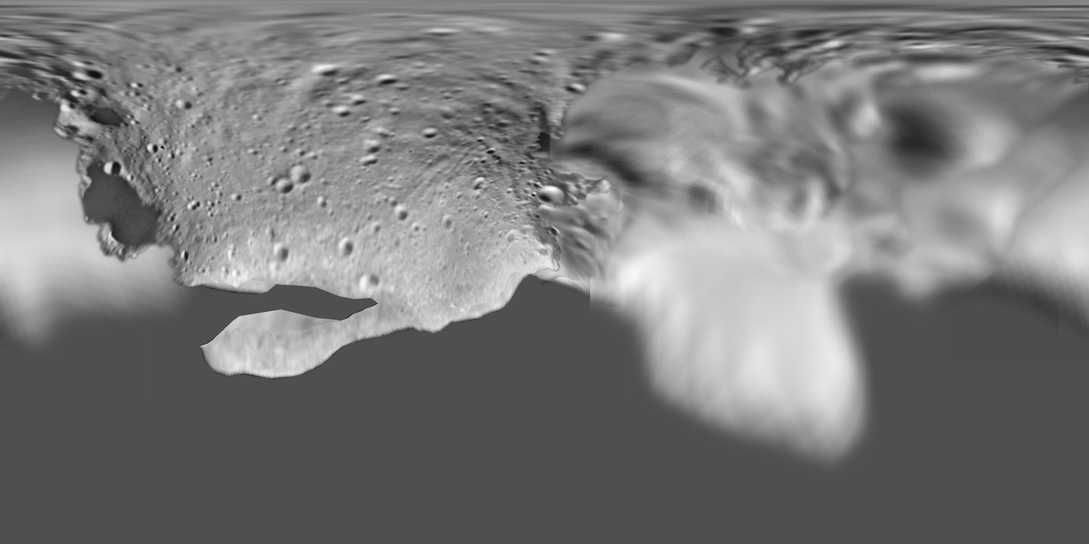
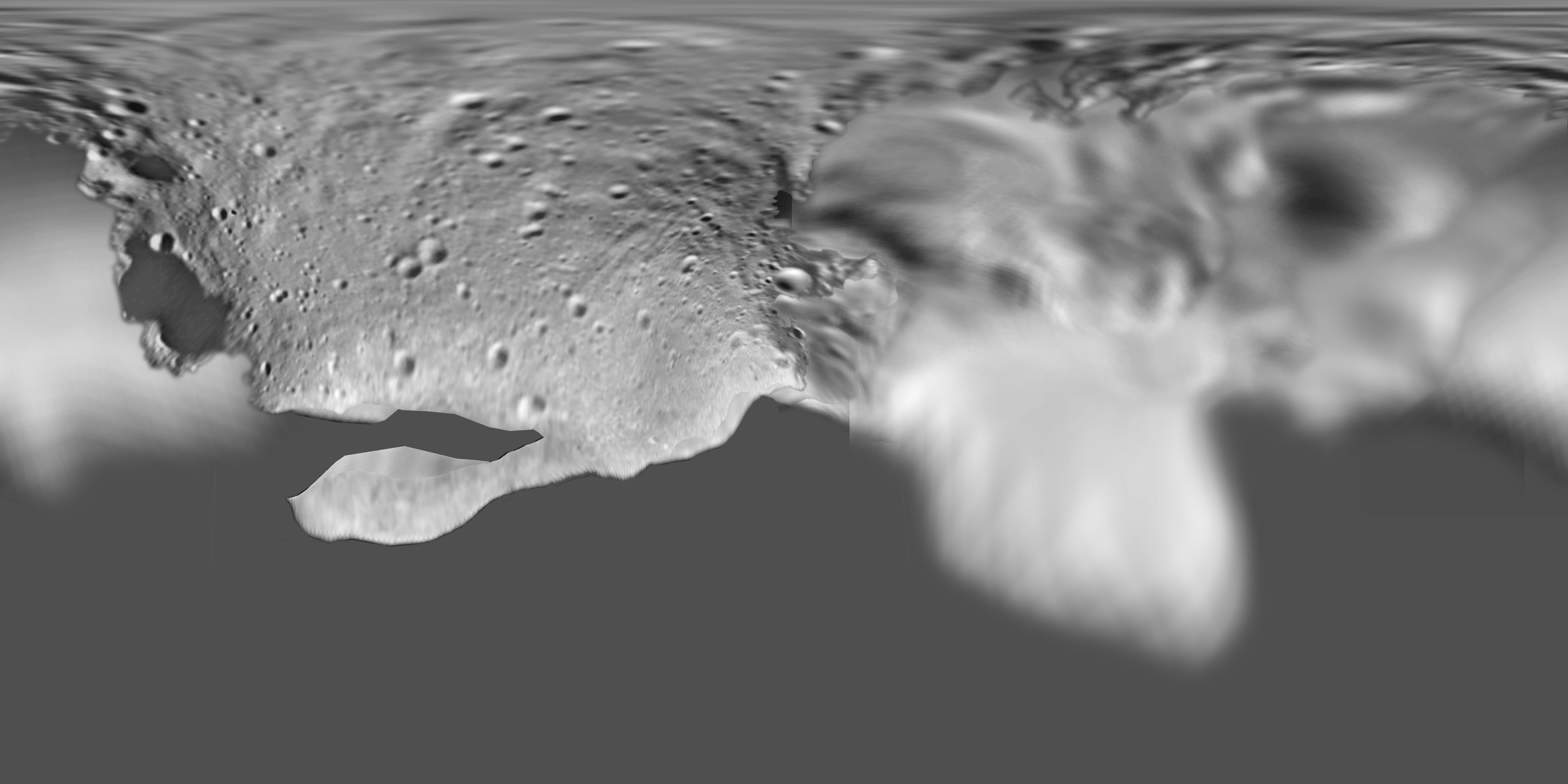
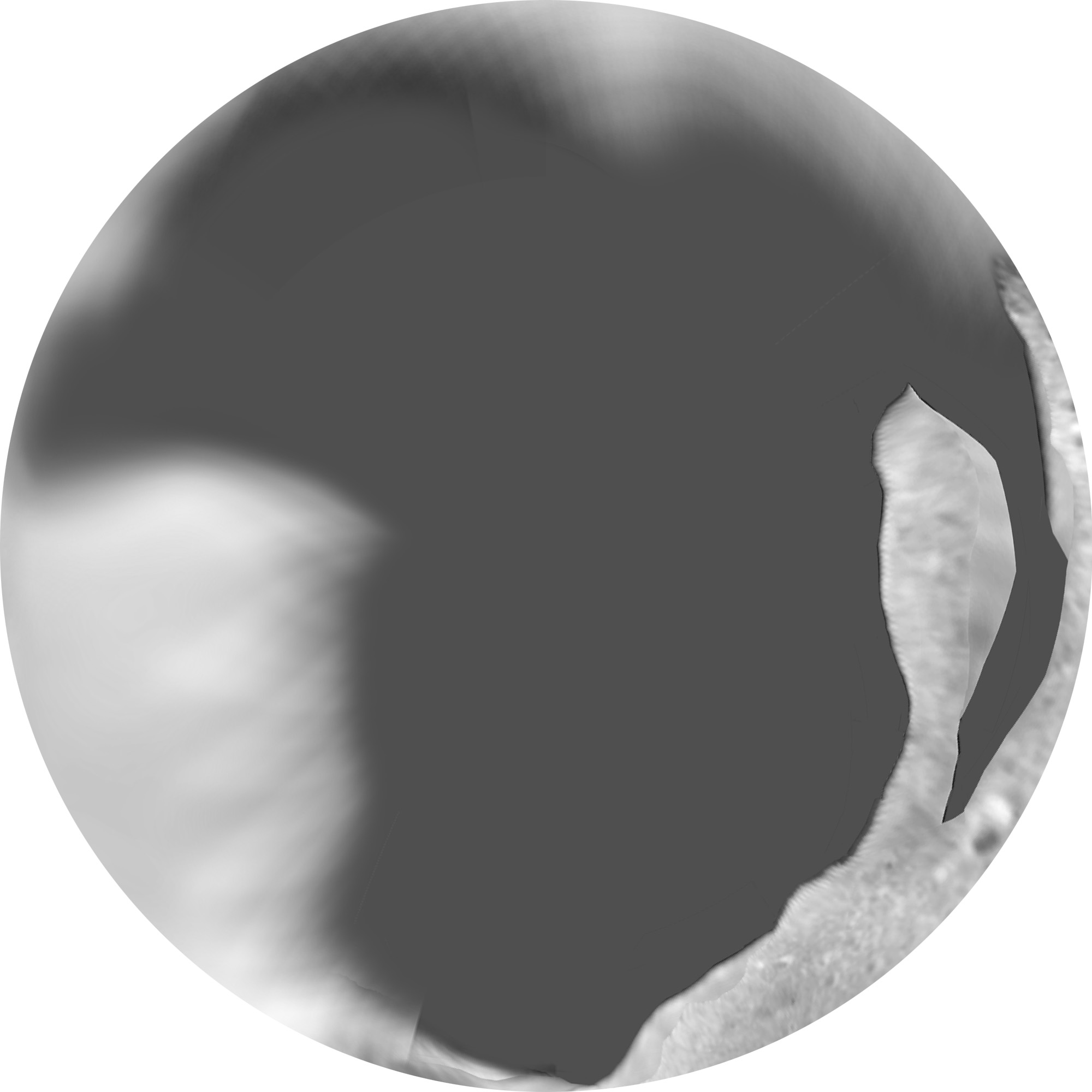
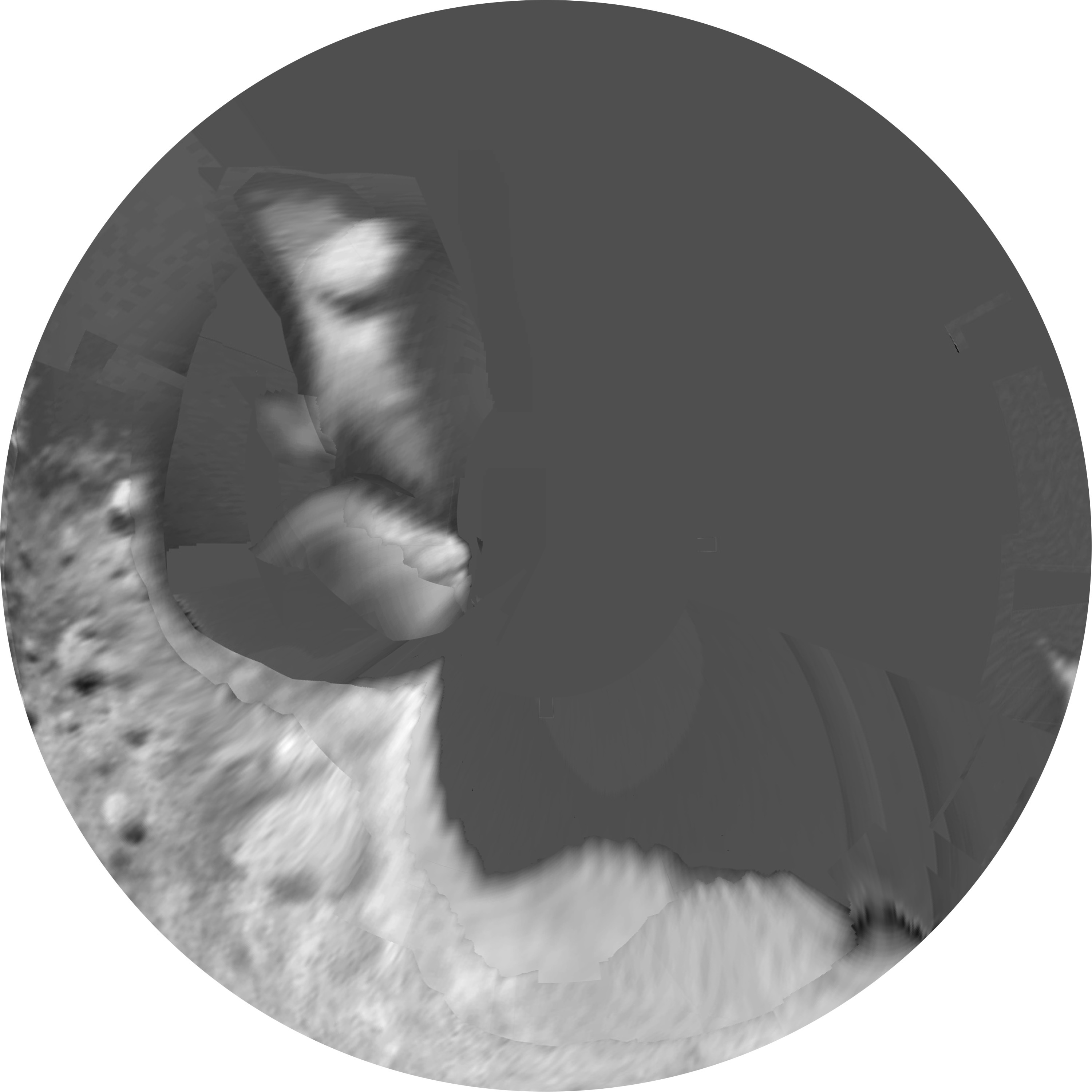
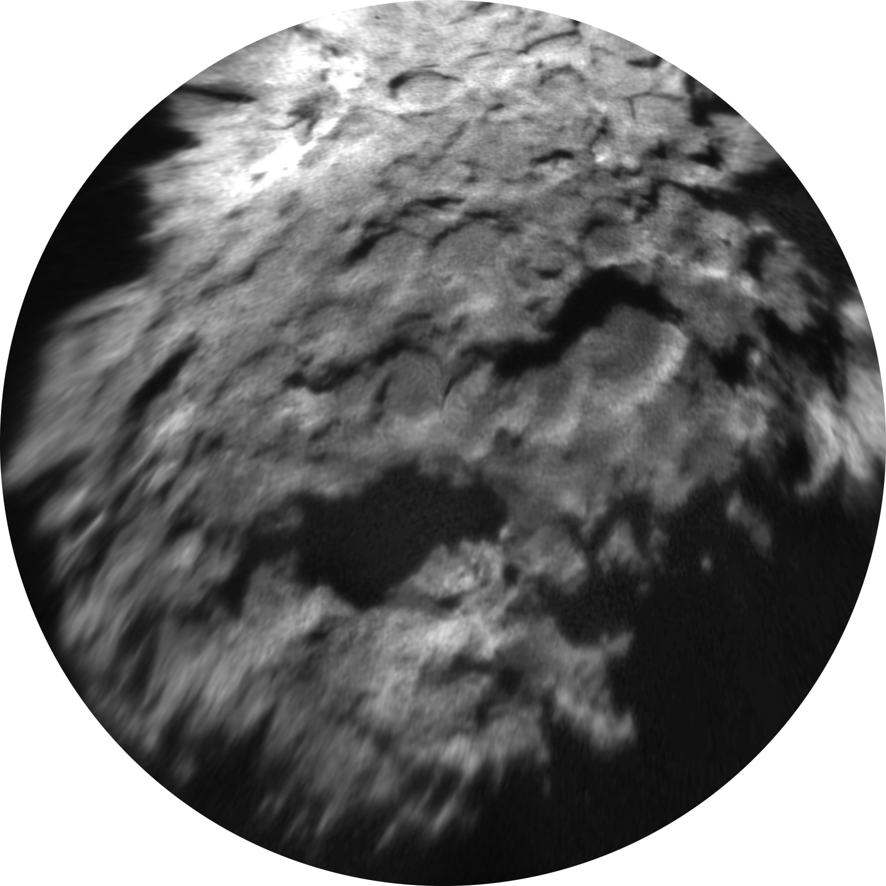
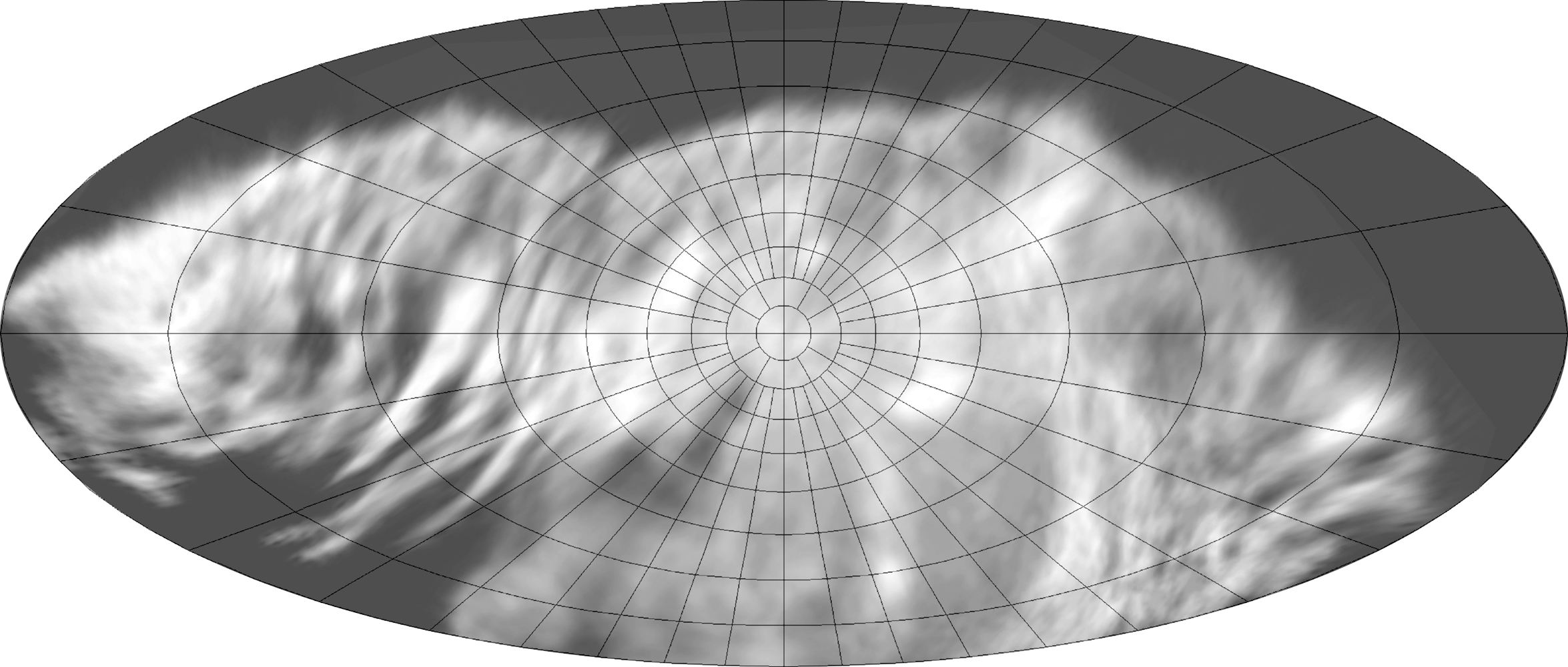
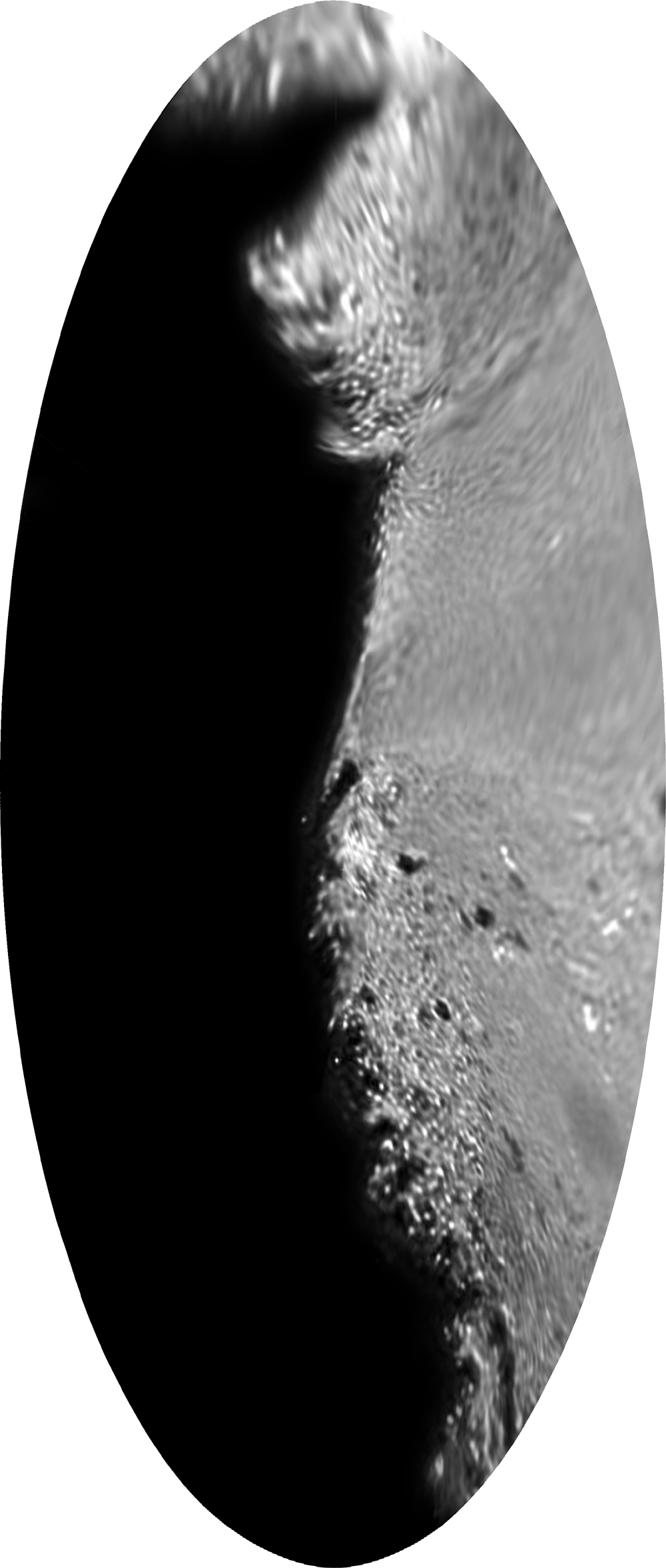
The mapping process involved two steps, each represented by a map in this dataset. First the gridded images from Hirata et al. (2009) were used to control reprojection of matching rendered images into a cylindrical projection. Those reprojections were combined to give full global coverage of Itokawa in cylindrical projection made up of a composite of the rendered images. This process fails in a small area near 30 degrees south on the prime meridian where a planetocentric radius cuts the surface several times (in effect, it is an overhanging cliff in planetocentric terms). In this small area there is no unambiguous relationship between the latitude-longitude-radius coordinate system and the x-y (or line-sample) coordinate system of the cylindrical projection. In this area the surface appears smeared and cannot be interpreted meaningfully. Nevertheless, the image provides a reasonable representation of the surface, allowing individual rocks or other features to be identified. It is offered here as an aid to visualization where a global map in conventional coordinates is required. The original rendered images will always be better for geometrically precise representation or measurements.
Simple Cylindrical Projection, north at the top, 0 longitude at the left and right edges, 180 degrees at the center, 7200 by 3600 pixels. (20 pixels/degree)
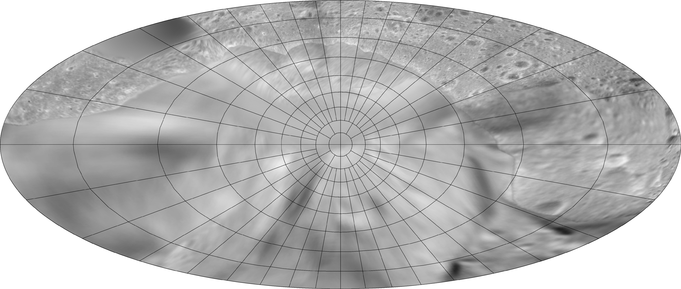
Same map, reduced and overlaid with a labelled grid.
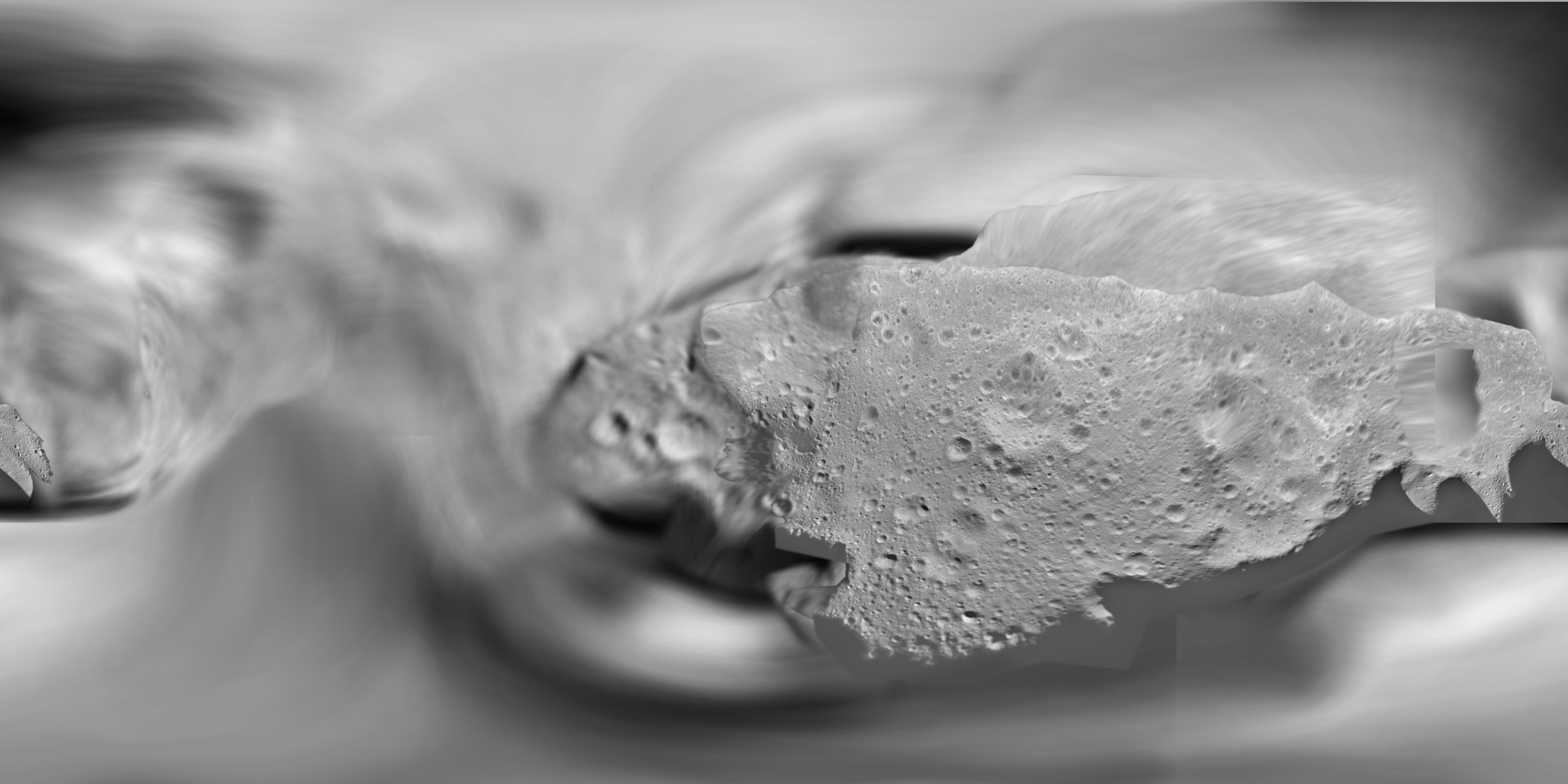
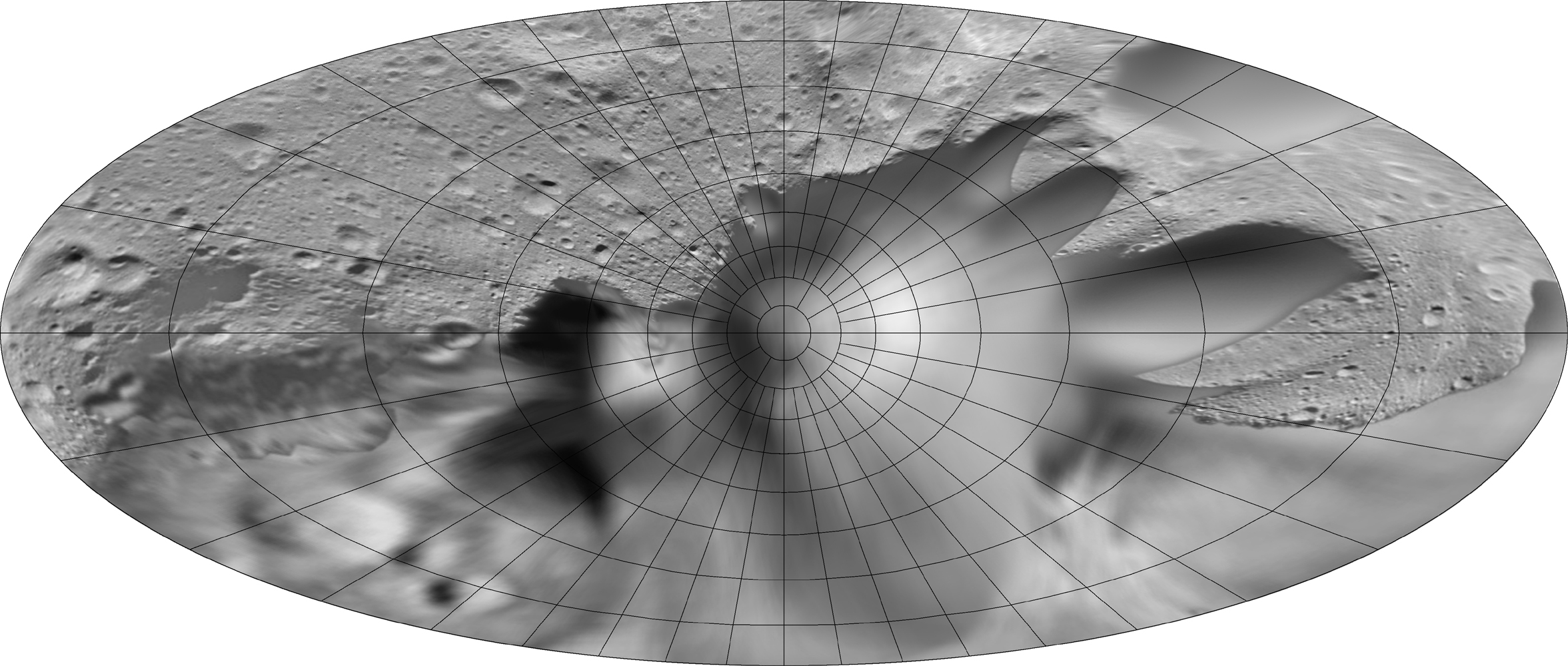
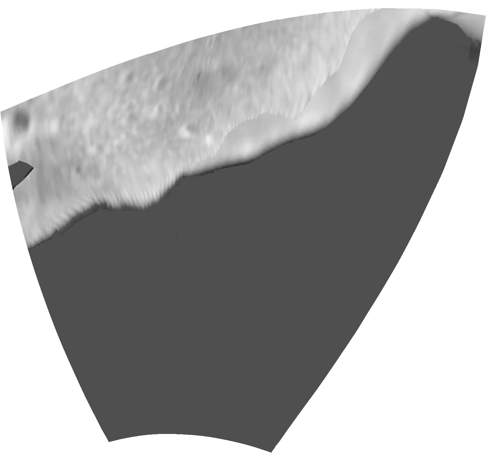
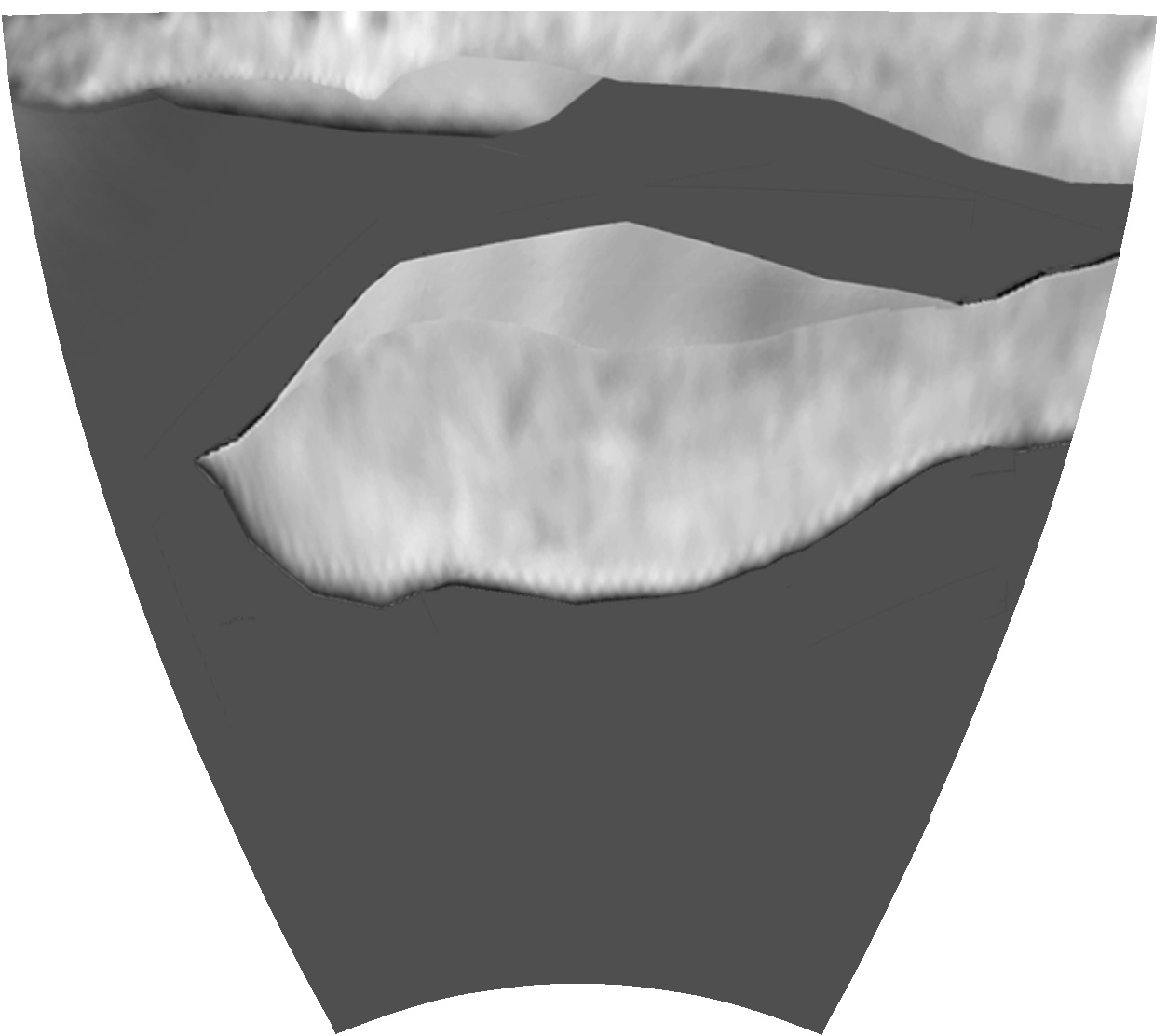
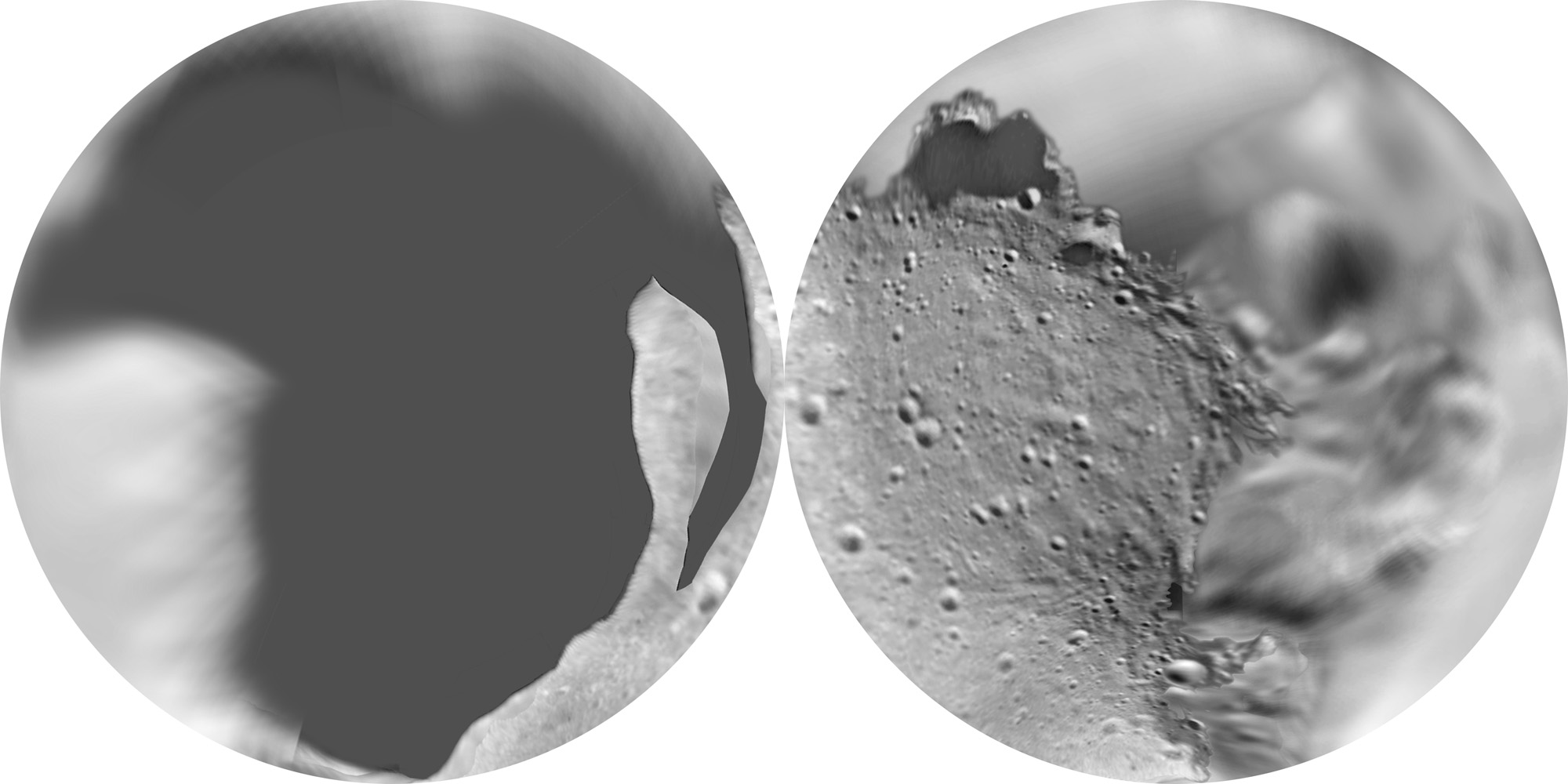
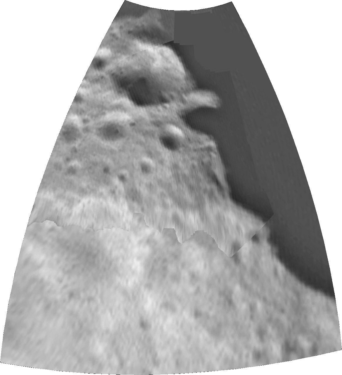
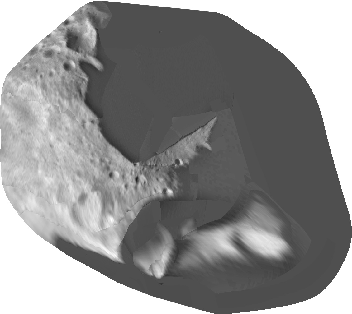
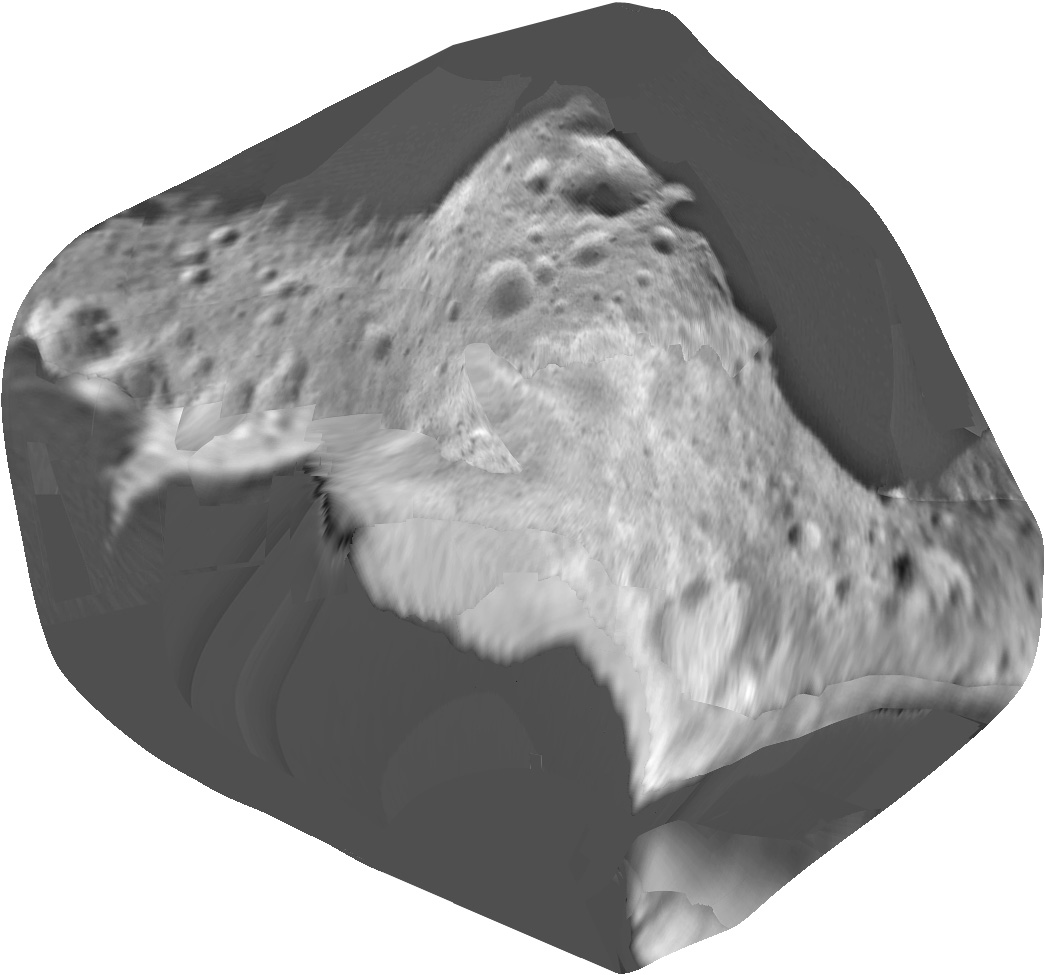
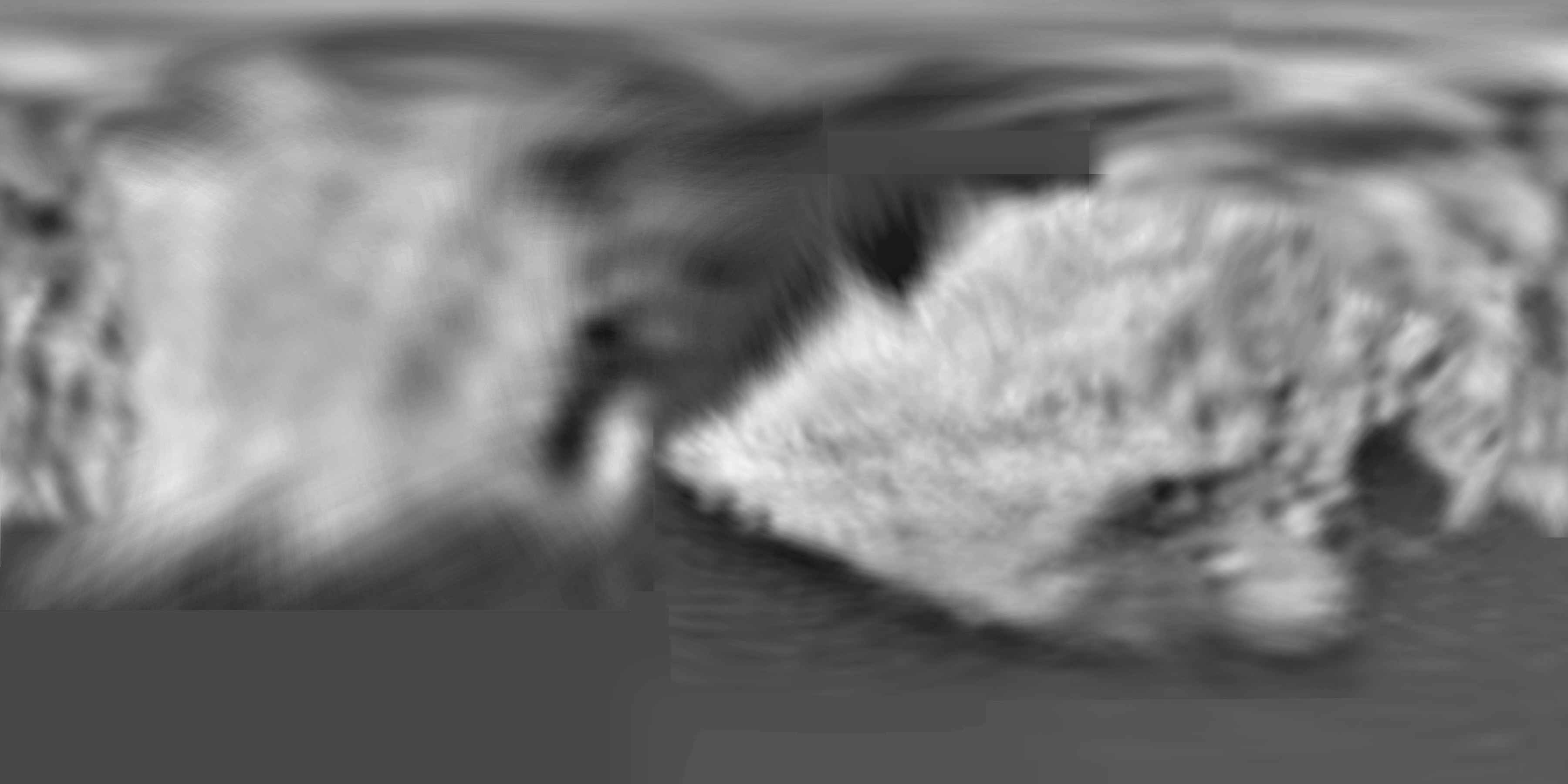
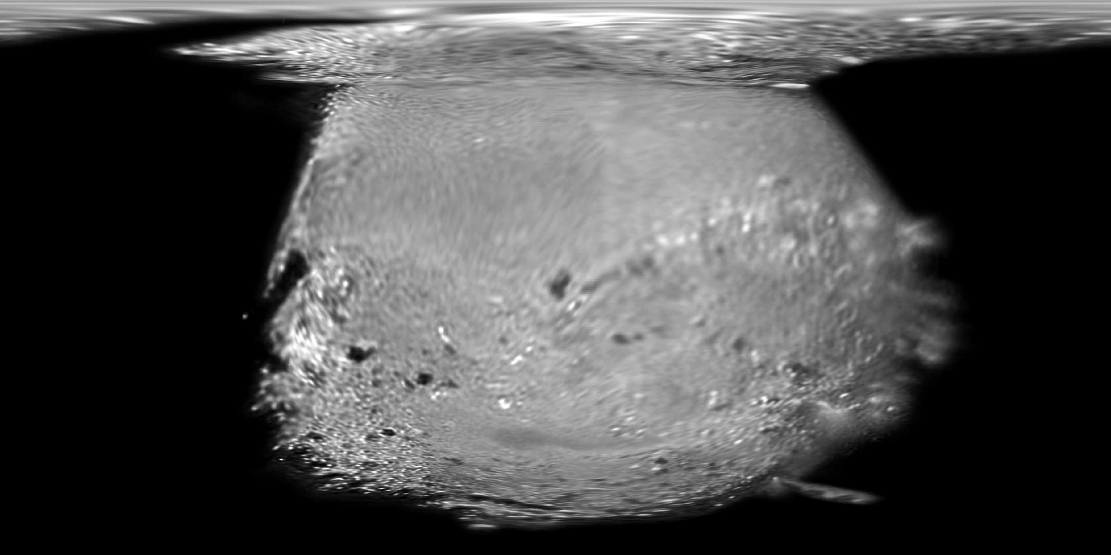
The second step replaces the computer-rendered image with a global photomosaic map. In each region across the asteroid, the best image was selected and reprojected to fit the cylindrical rendered image using small rocks as control points. A composite global mosaic was constructed with lighting as uniform as possible, though complete uniformity is impossible given limitations of the image data. Special care has been taken to map the problem area described above to improve visualizations in that region. Small dark areas on the 0 and 180 meridians in the southern hemisphere were never seen illuminated in Hayabusa images.
Both maps have the same geometry:
Simple Cylindrical Projection, north at the top, 0 longitude at the left and right edges, 180 degrees at the center, 7200 by 3600 pixels. (20 pixels/degree)
References:
Gaskell, R., Saito, J., Ishiguro, M., Kubota, T., Hashimoto, T., Hirata, N., Abe, S., Barnouin-Jha, O., and Scheeres, D., Gaskell Itokawa Shape Model V1.0. HAY-A-AMICA-5-ITOKAWASHAPE-V1.0. NASA Planetary Data System, 2008. (Available online)
Hirata, N., O.S. Barnouin-Jha, C. Honda, R. Nakamura, H. Miyamoto, S. Sasaki, H. Demura, A.M. Nakamura, T. Michikami, R.W. Gaskell, and J. Saito, A survey of possible impact structures on 25143 Itokawa, Icarus 200, 486-502 2009.
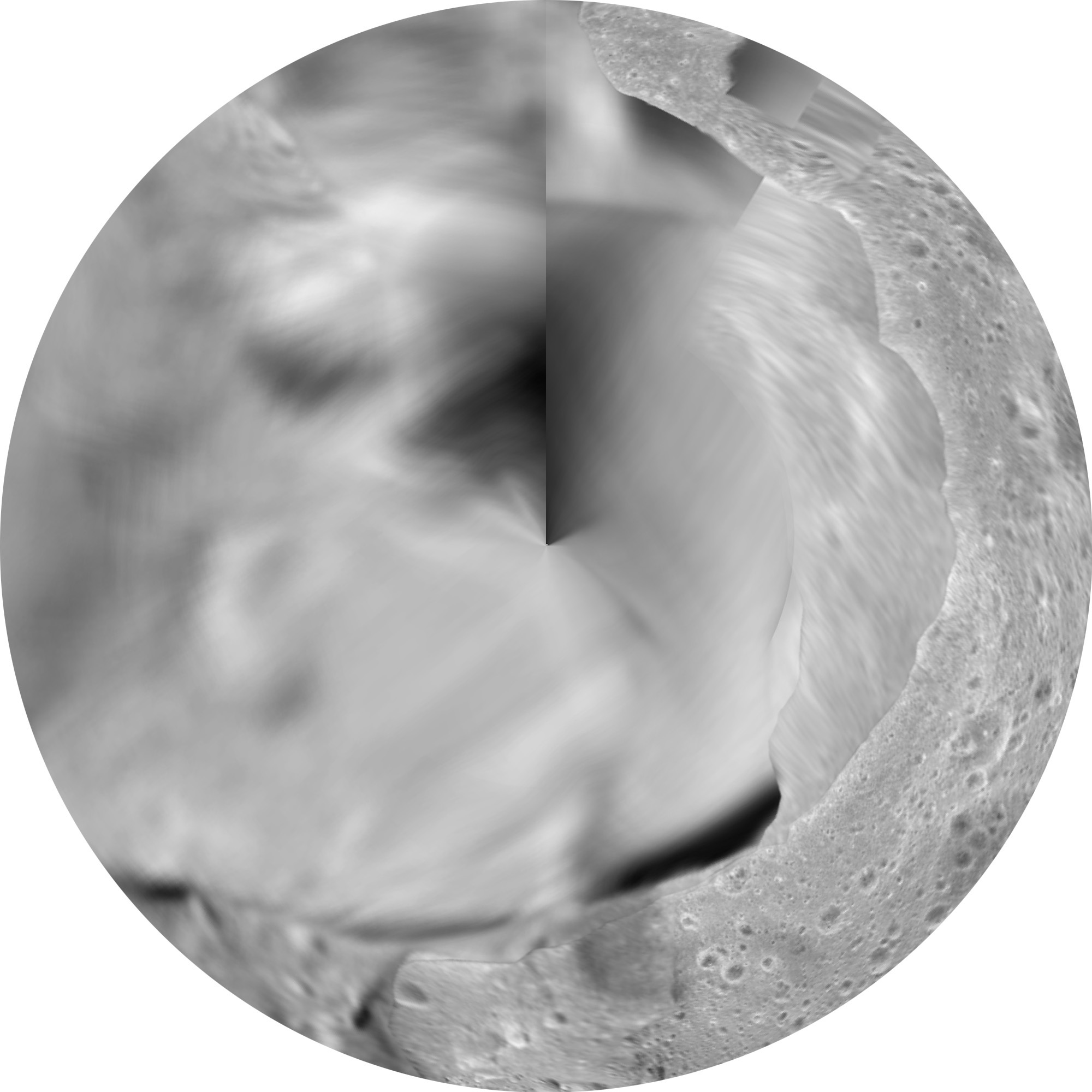
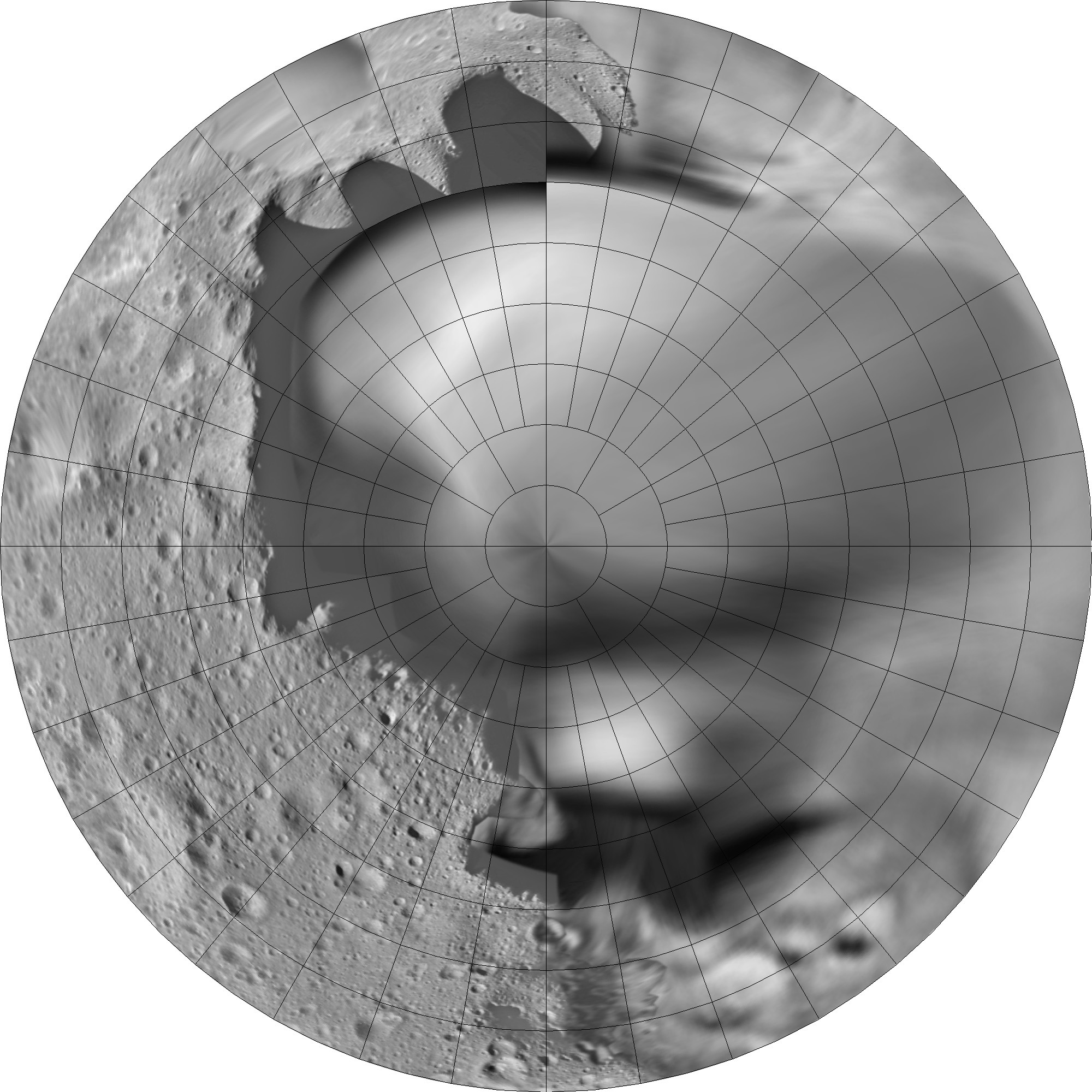
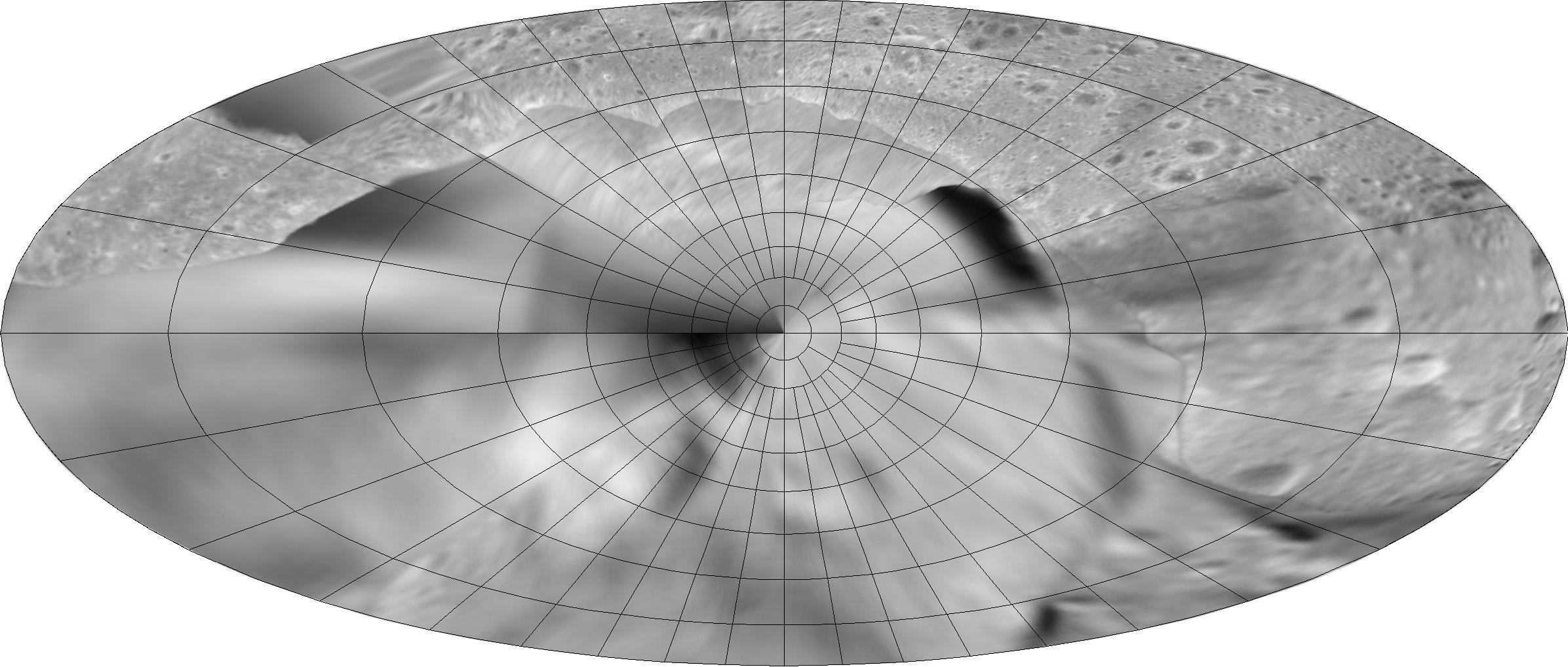
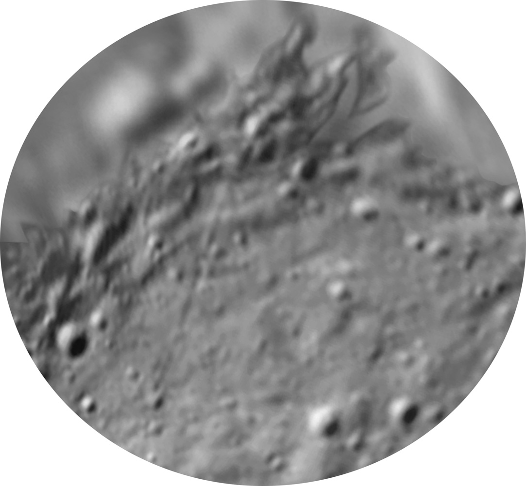
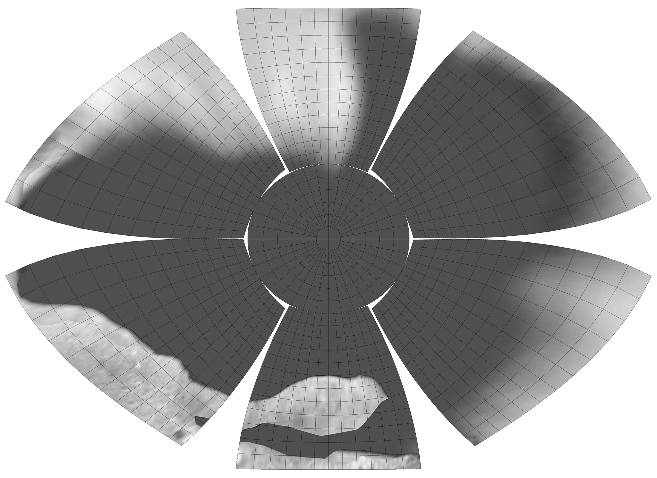
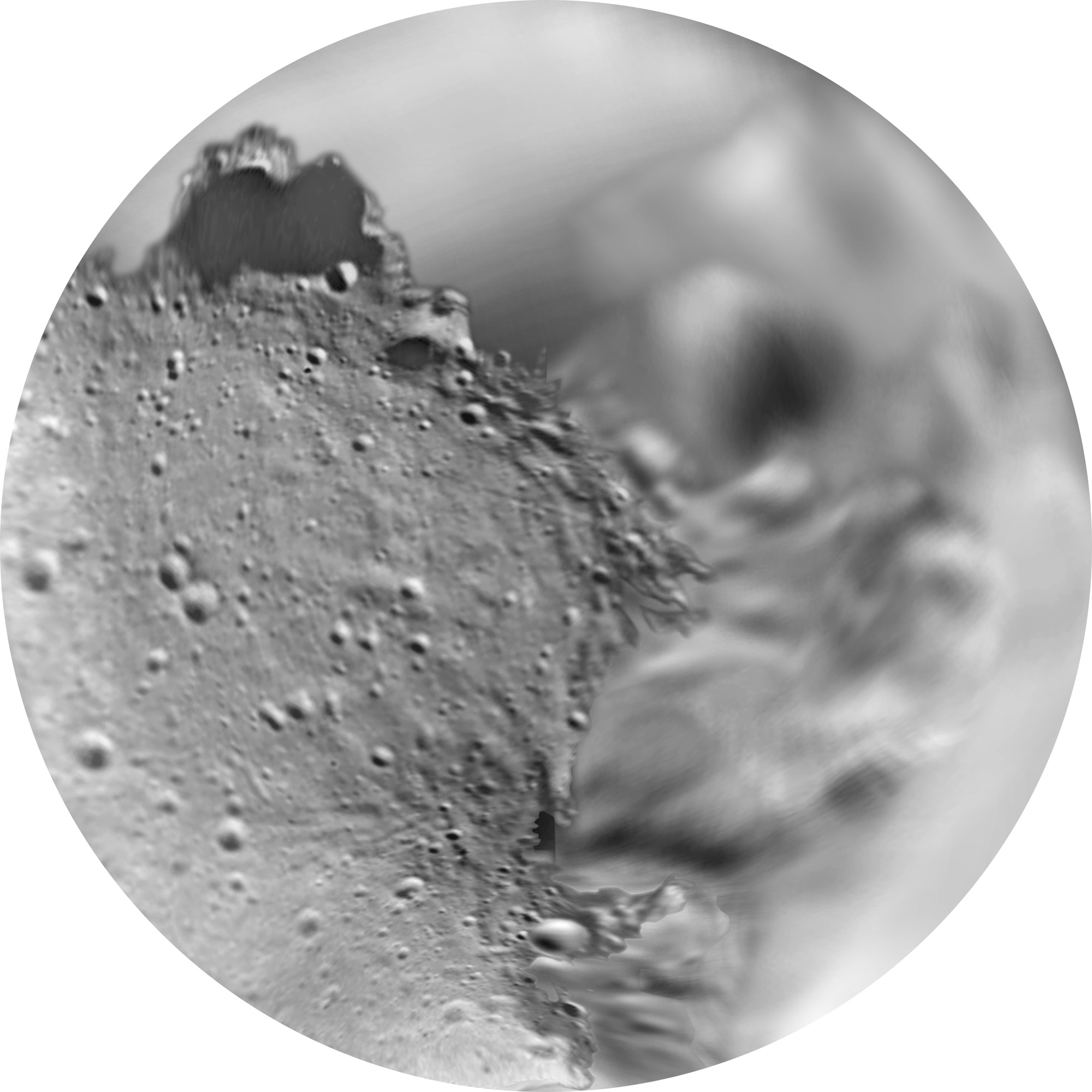
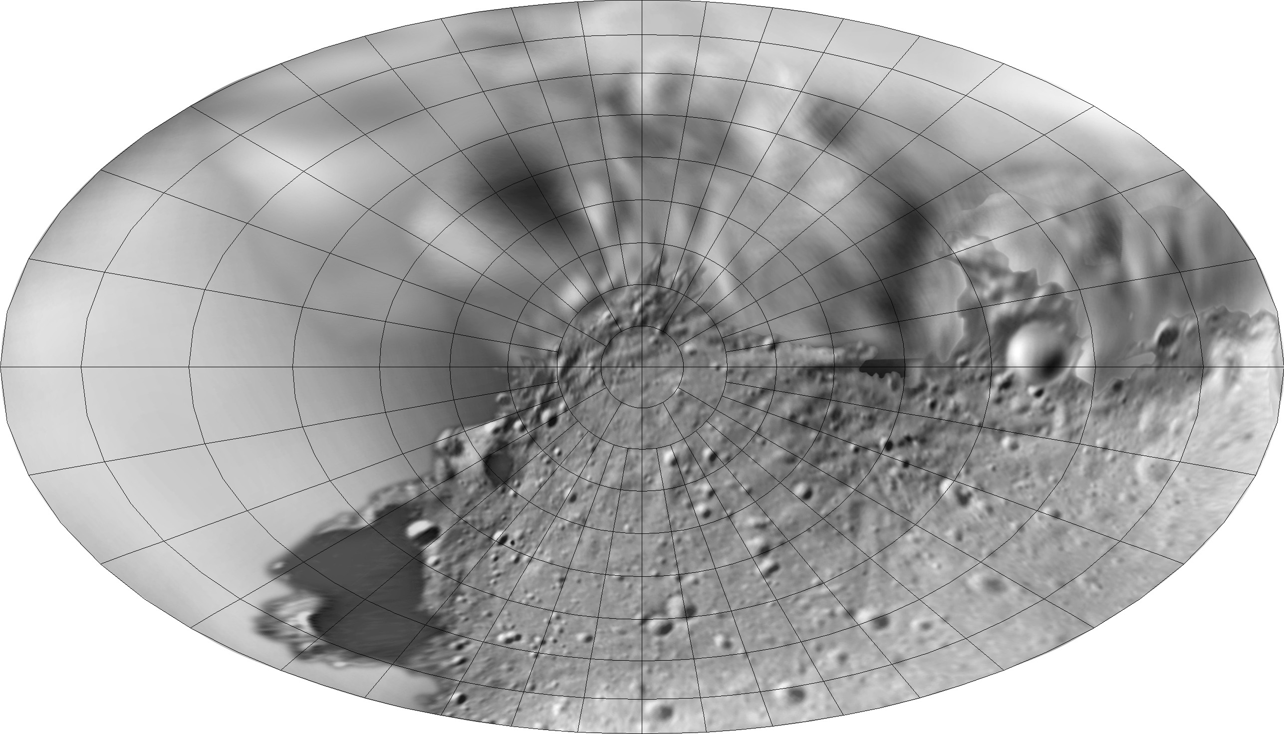
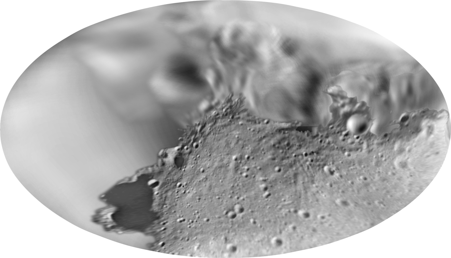
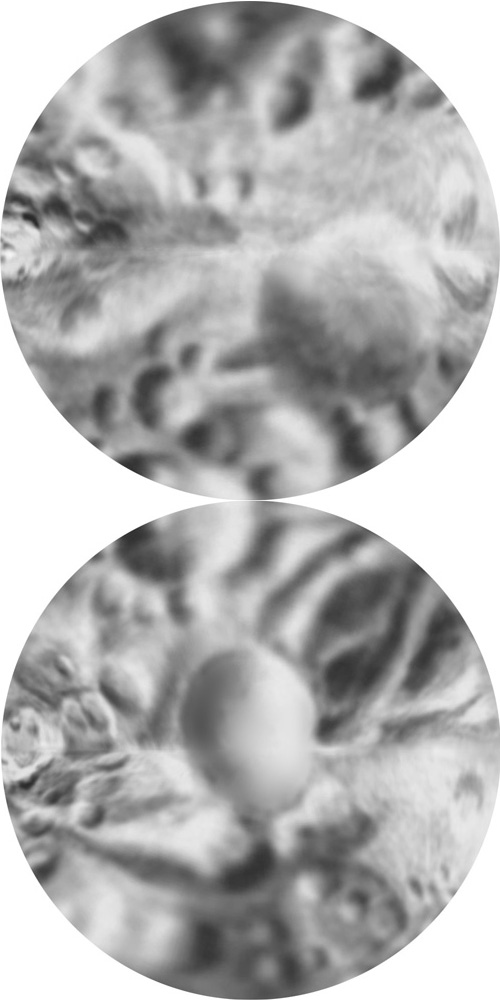
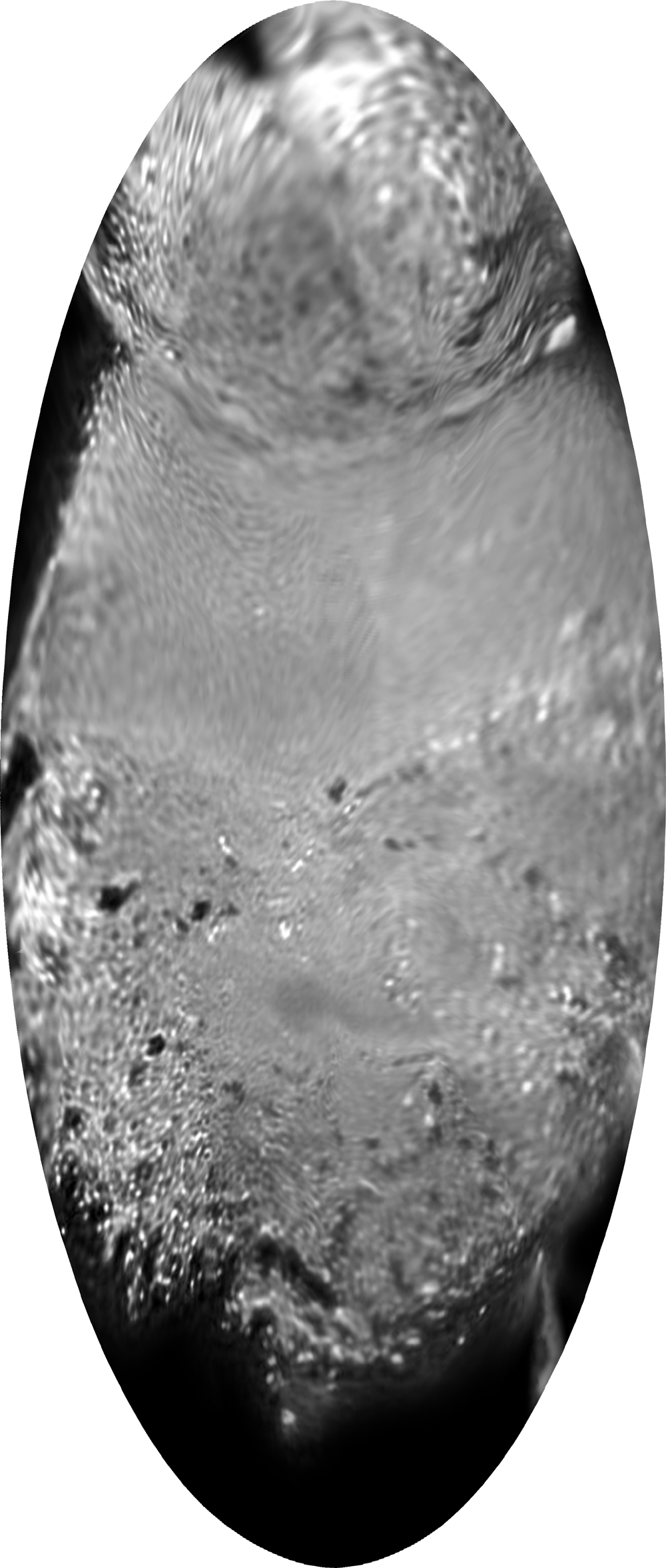
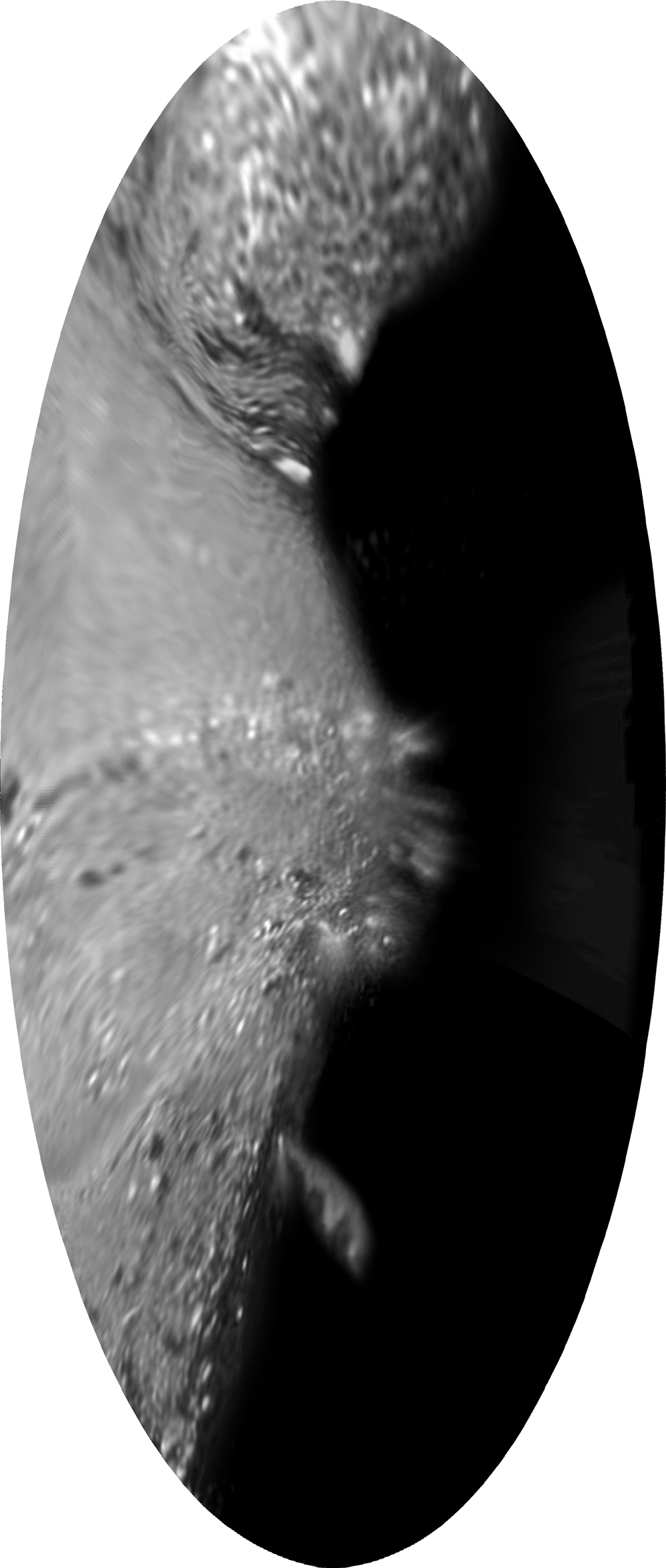
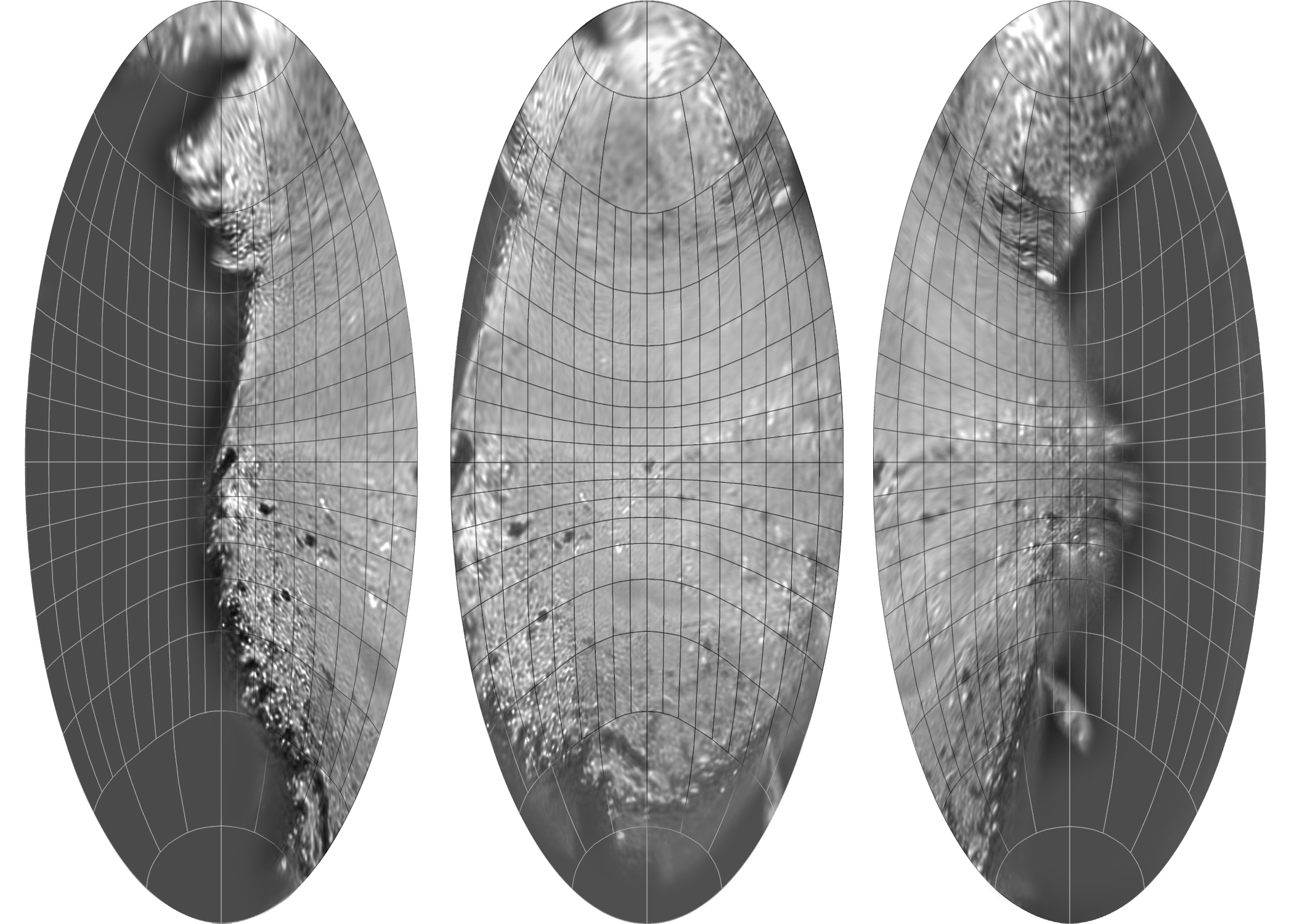
The following are reprojected ellipsoidal maps made from the cylindrical projection map above.
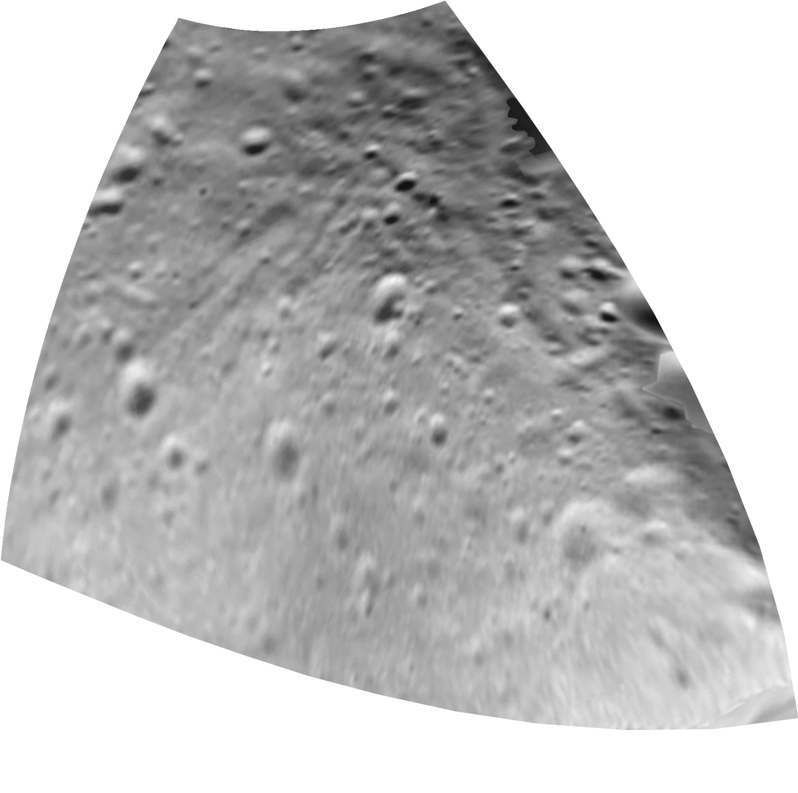
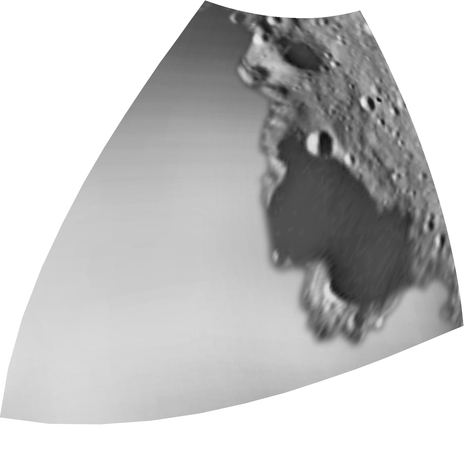
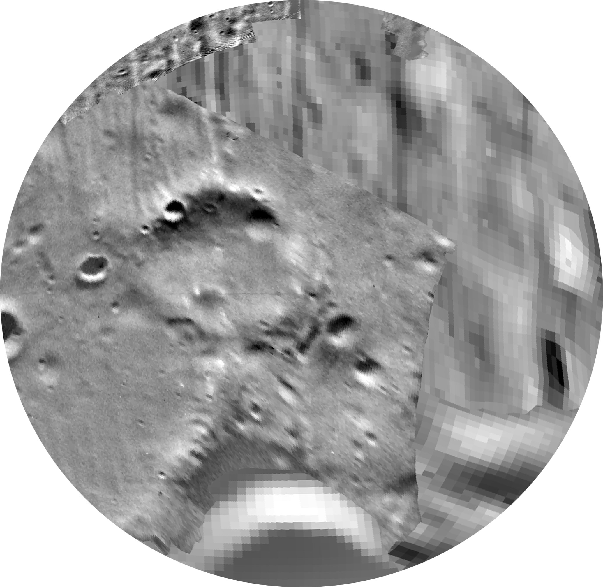
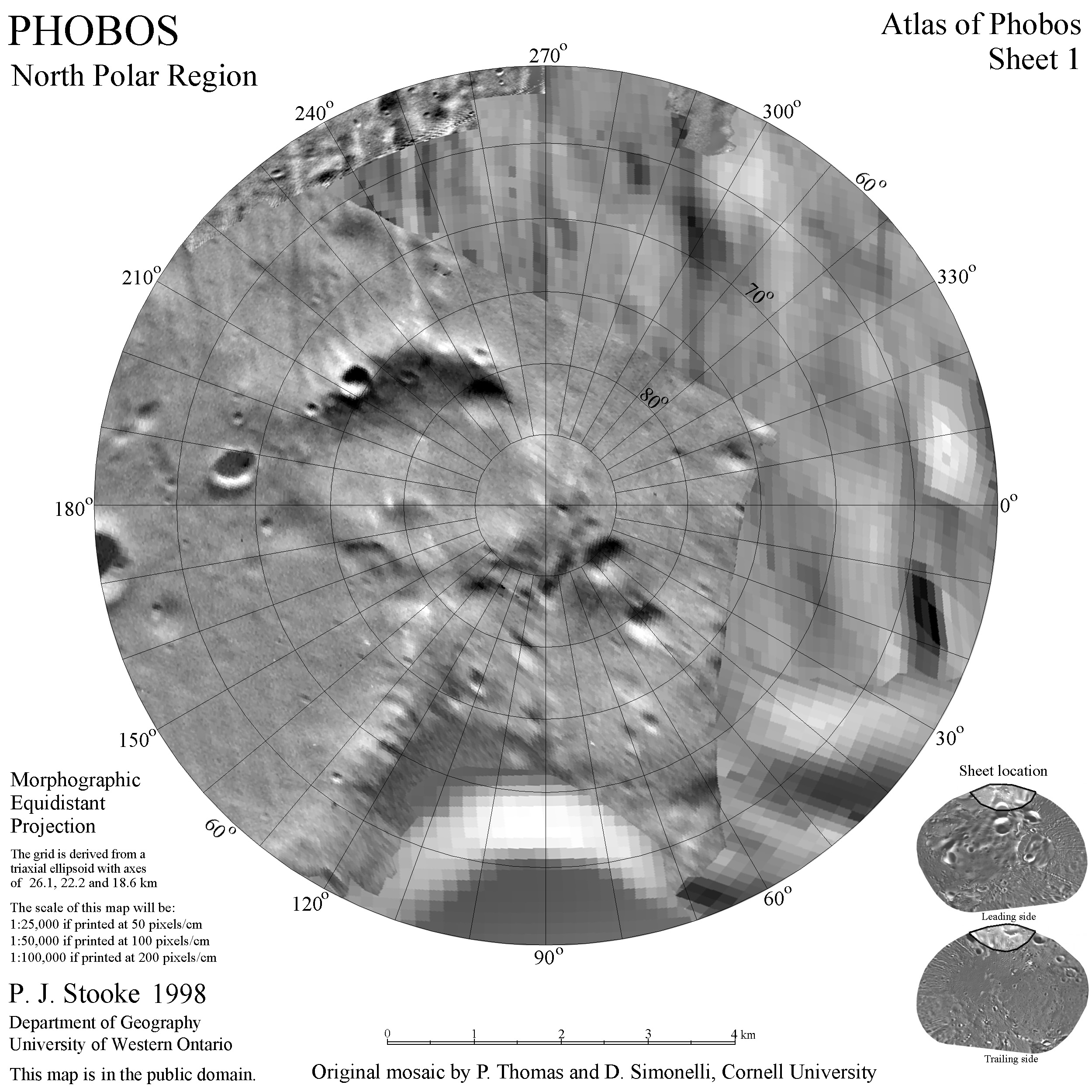
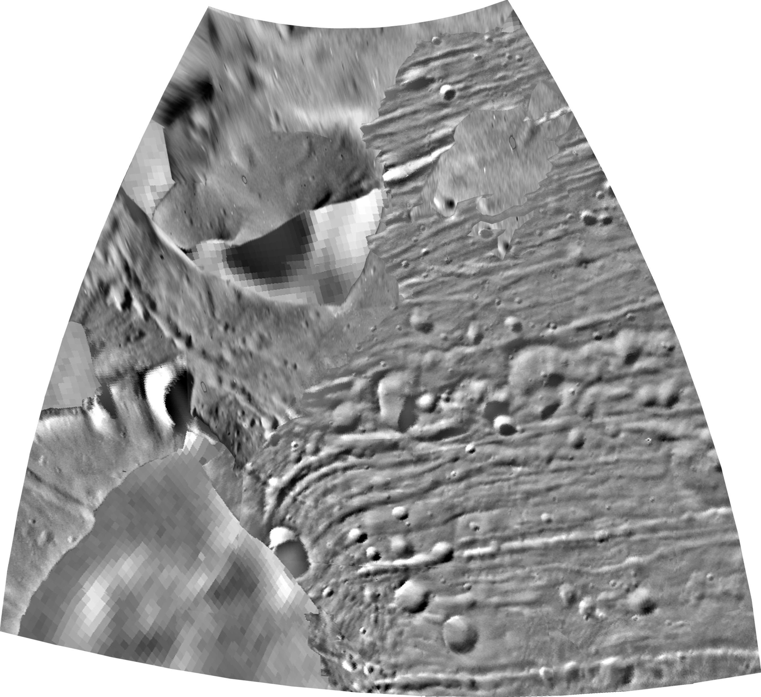
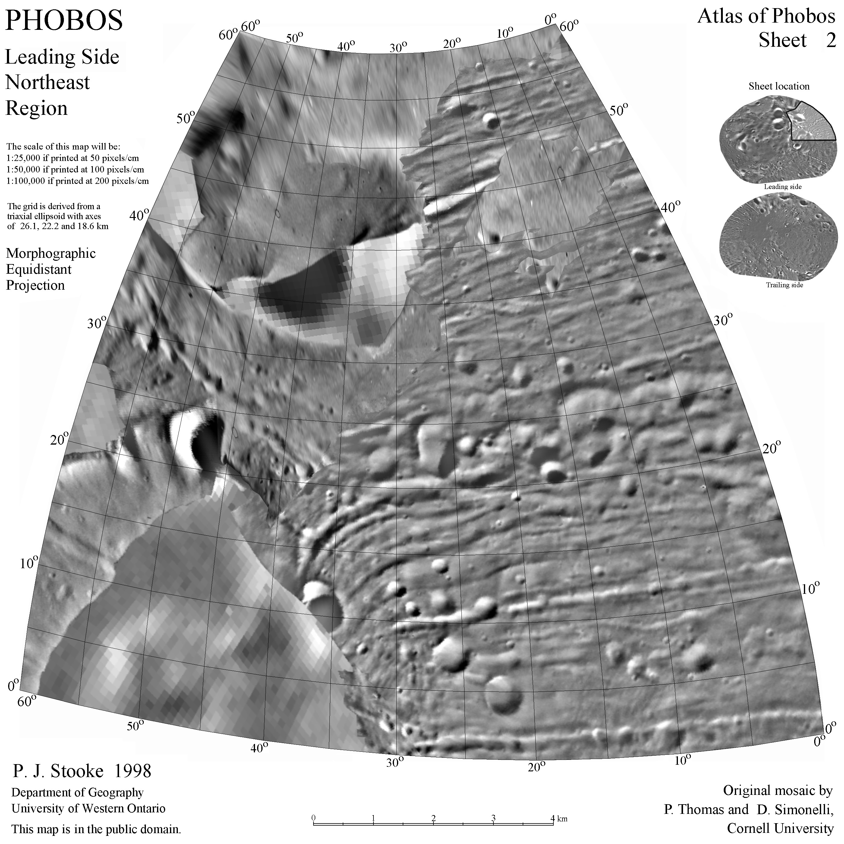
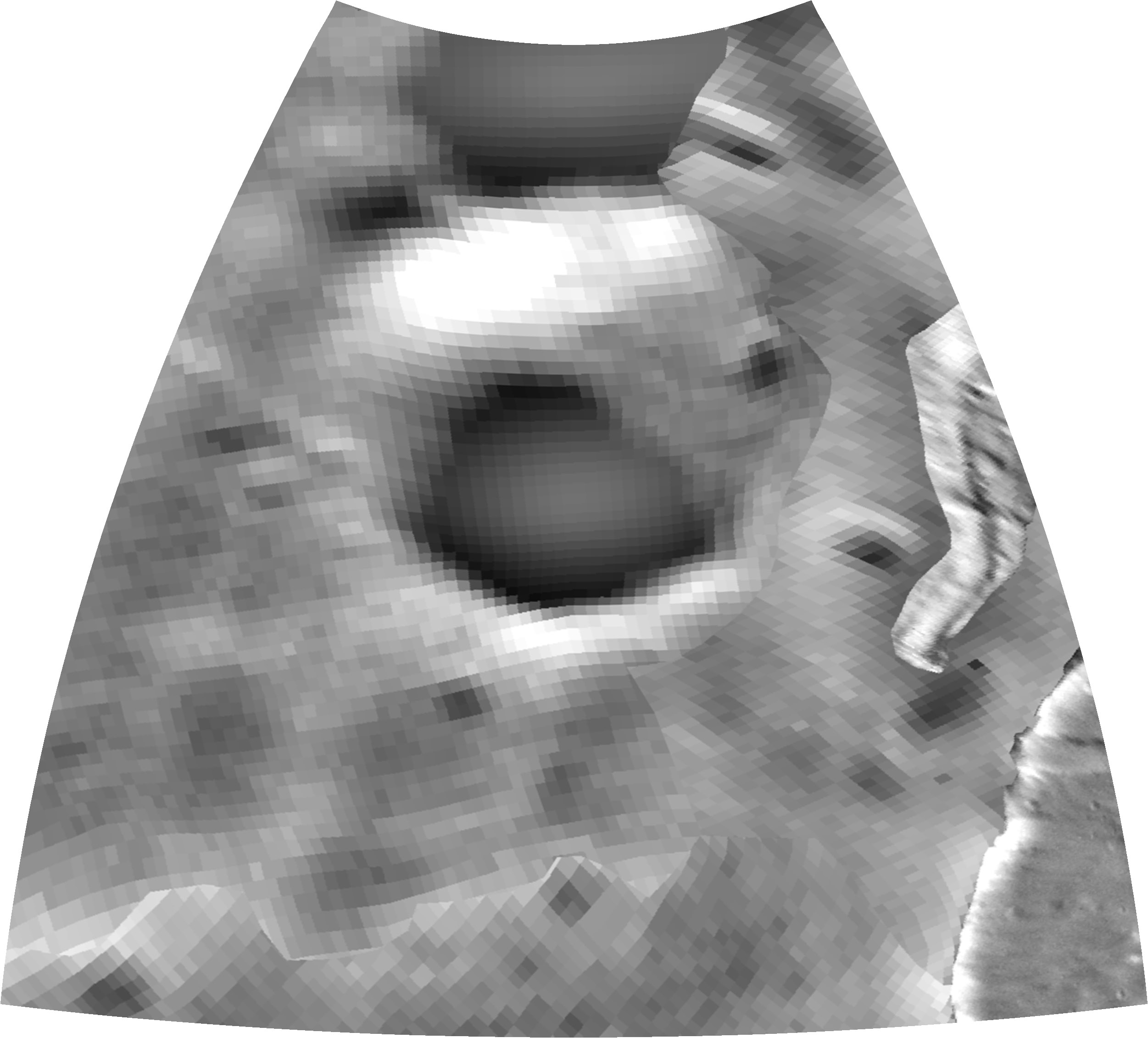
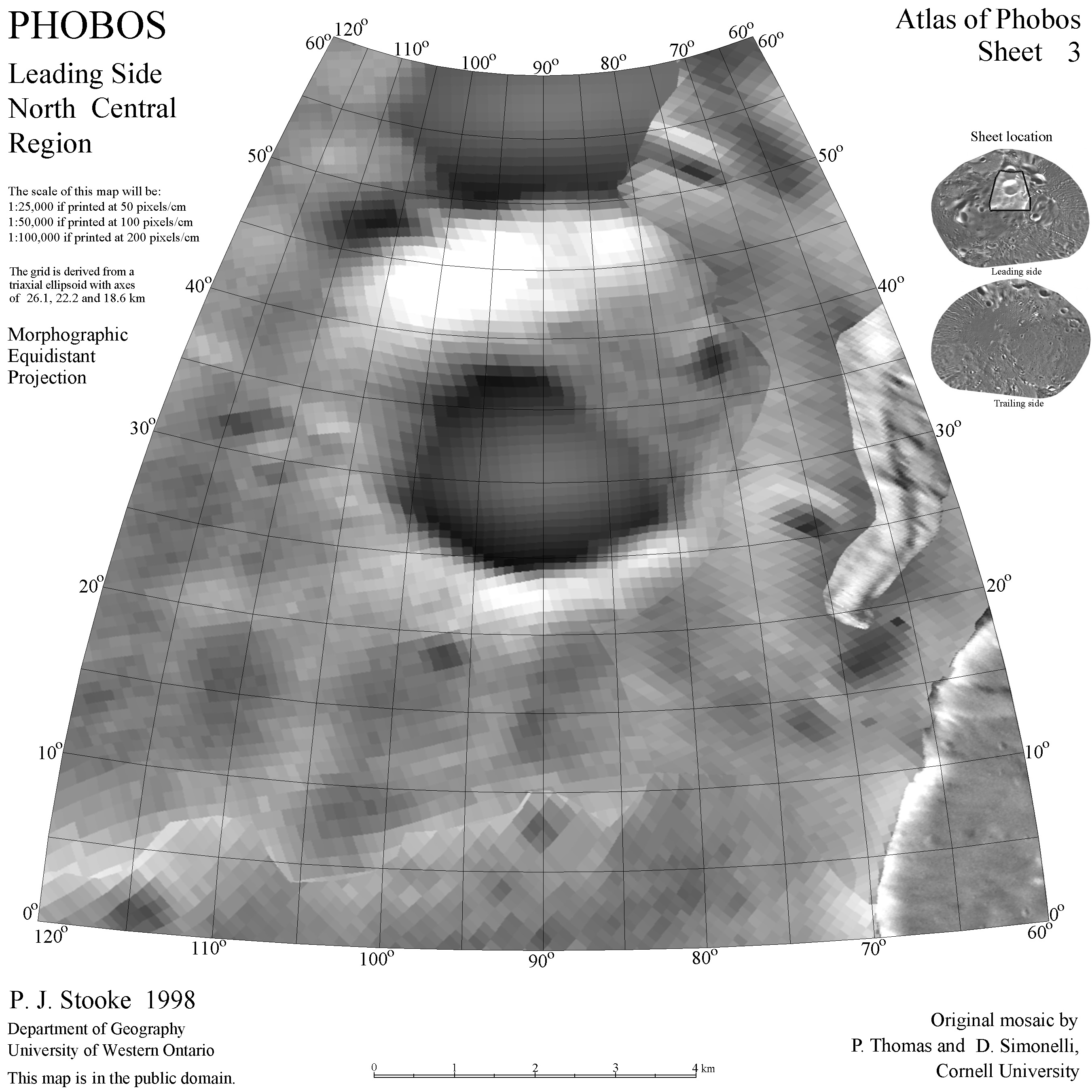
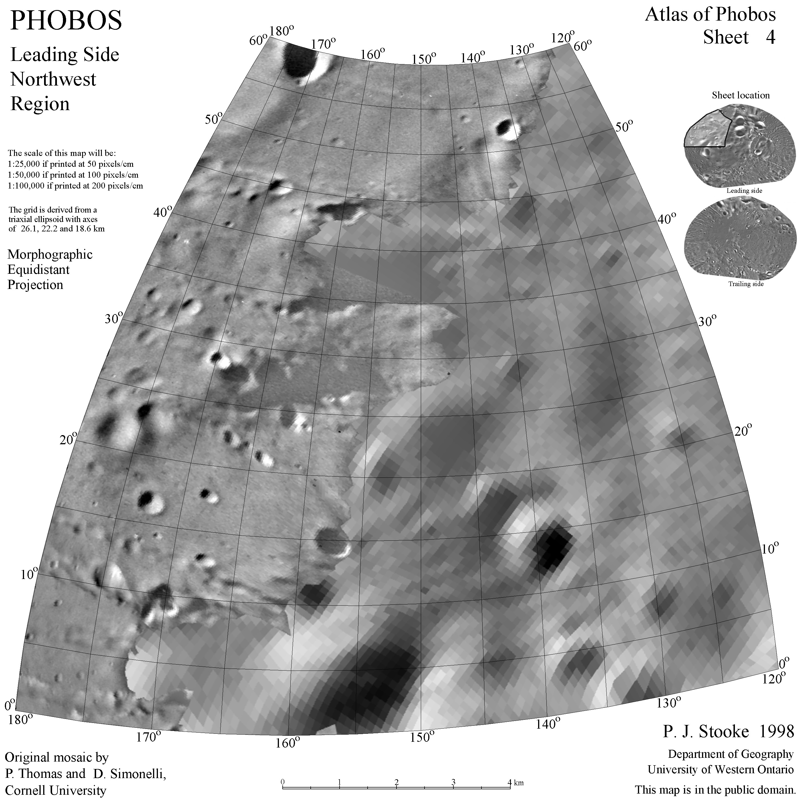
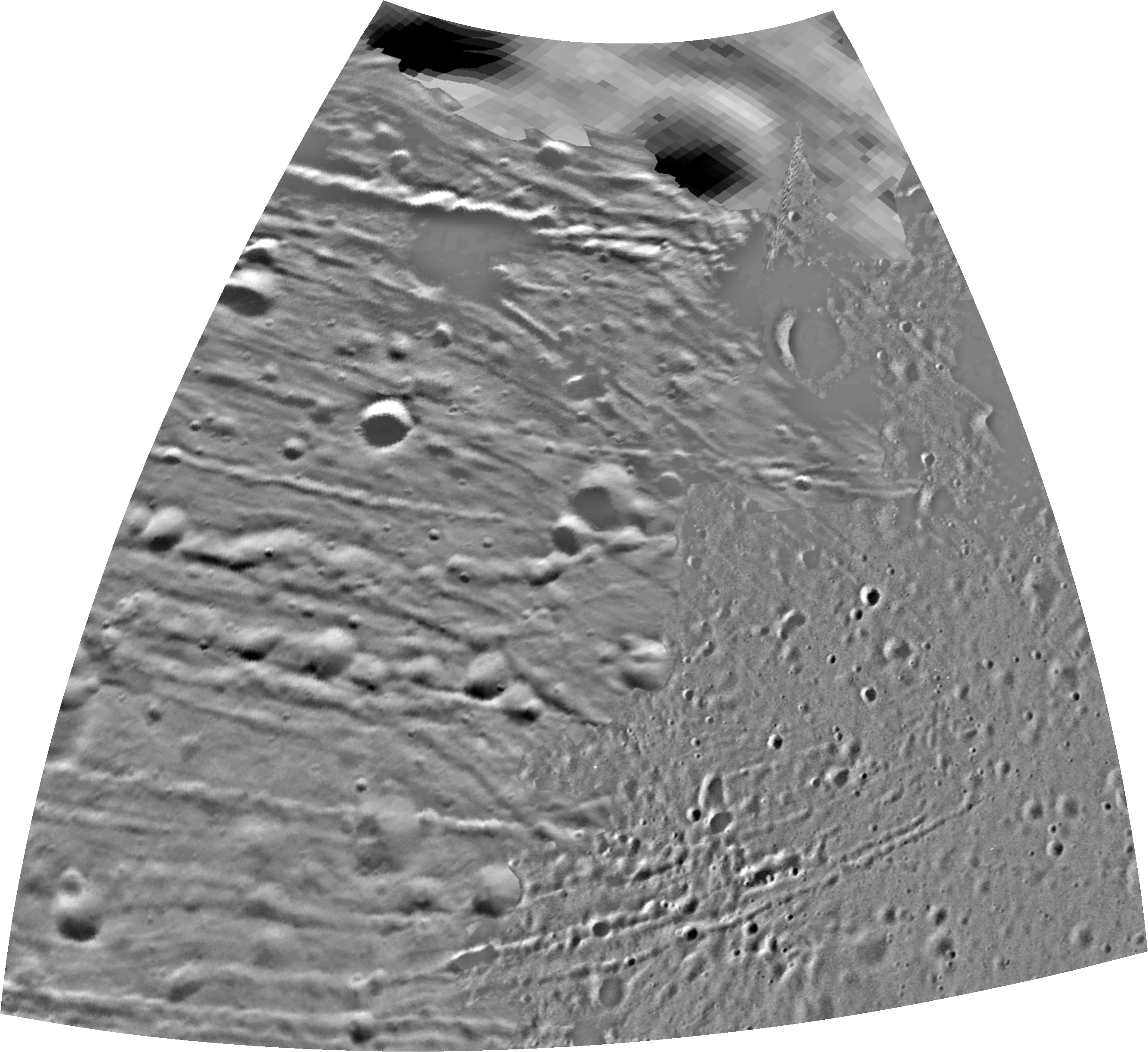
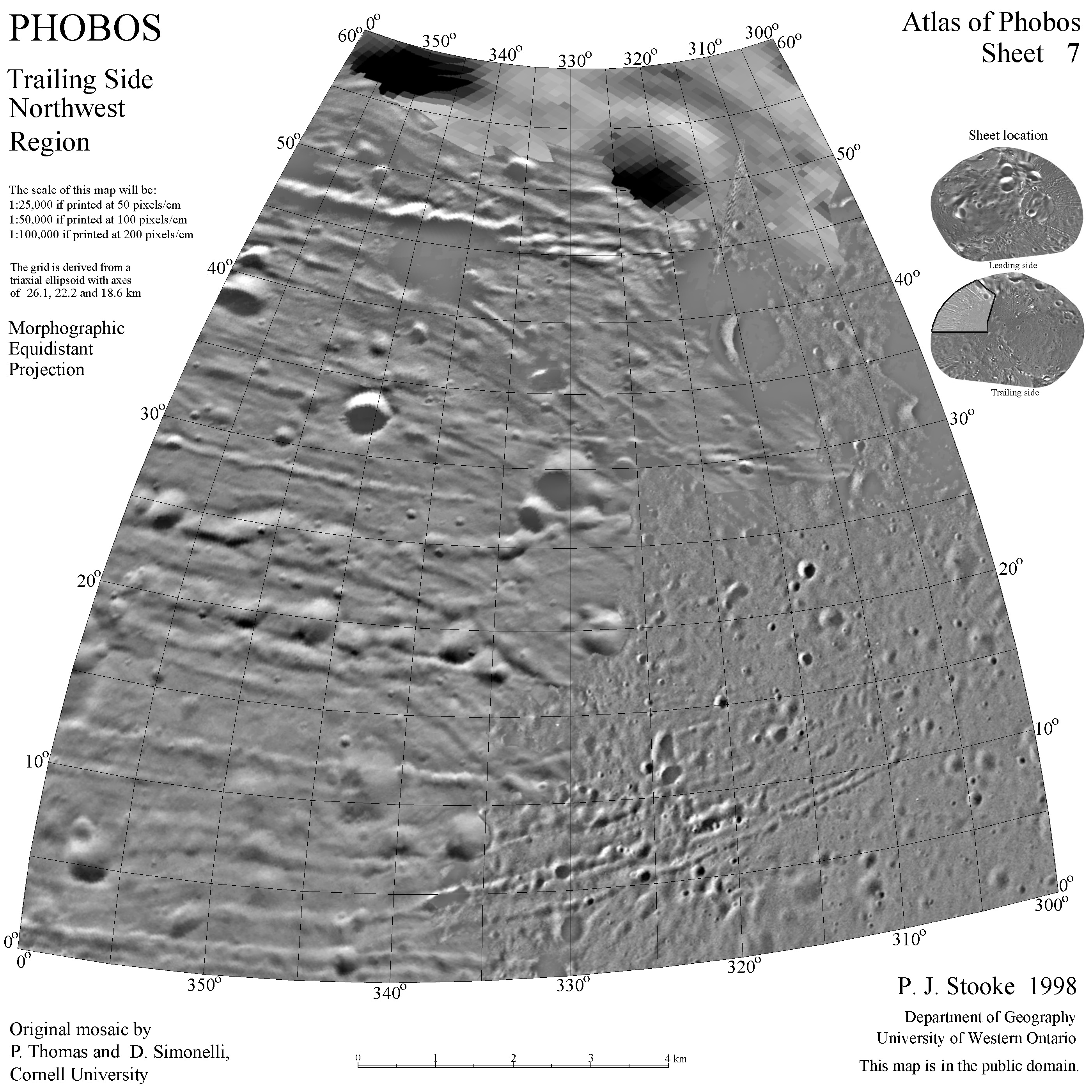
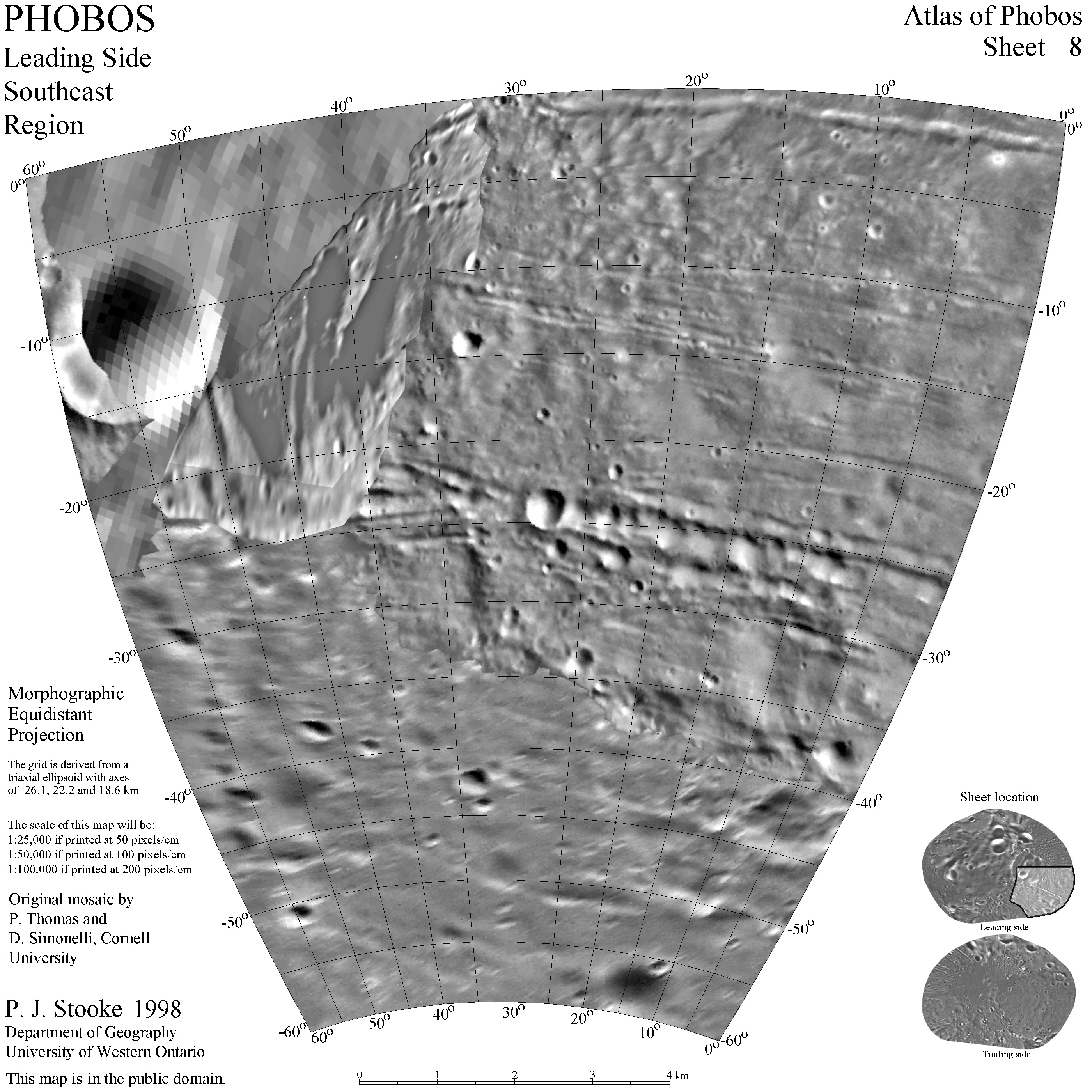
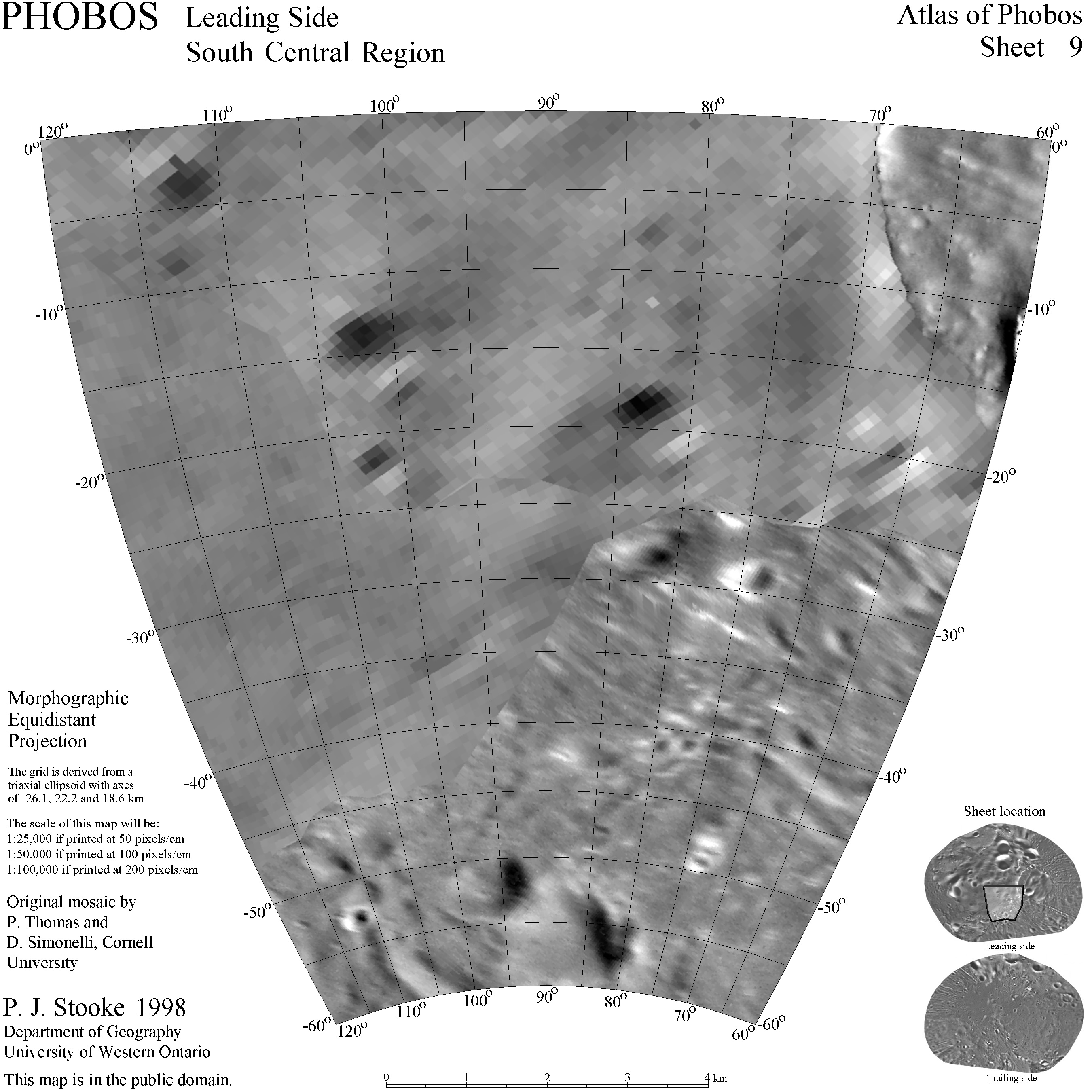
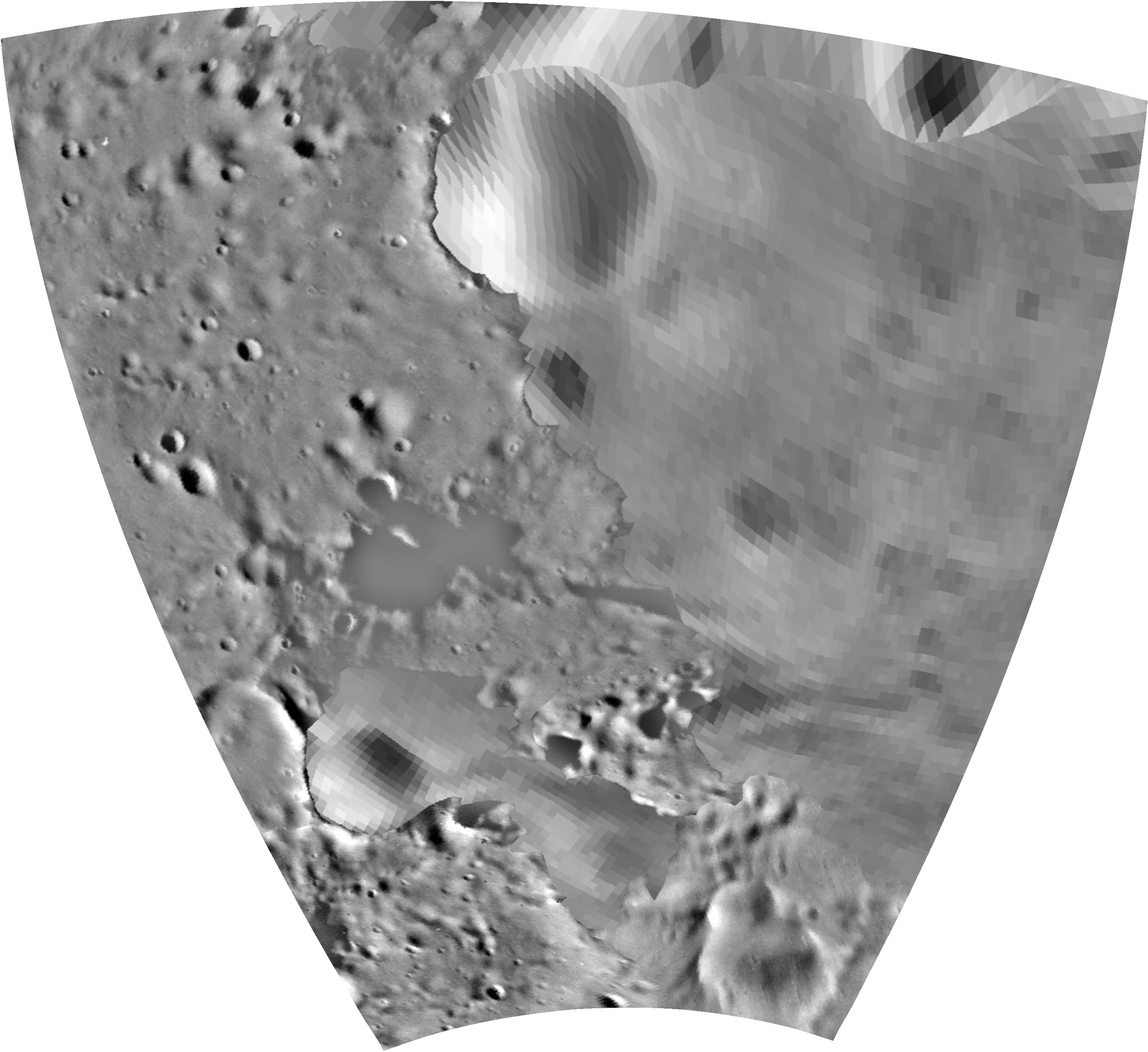
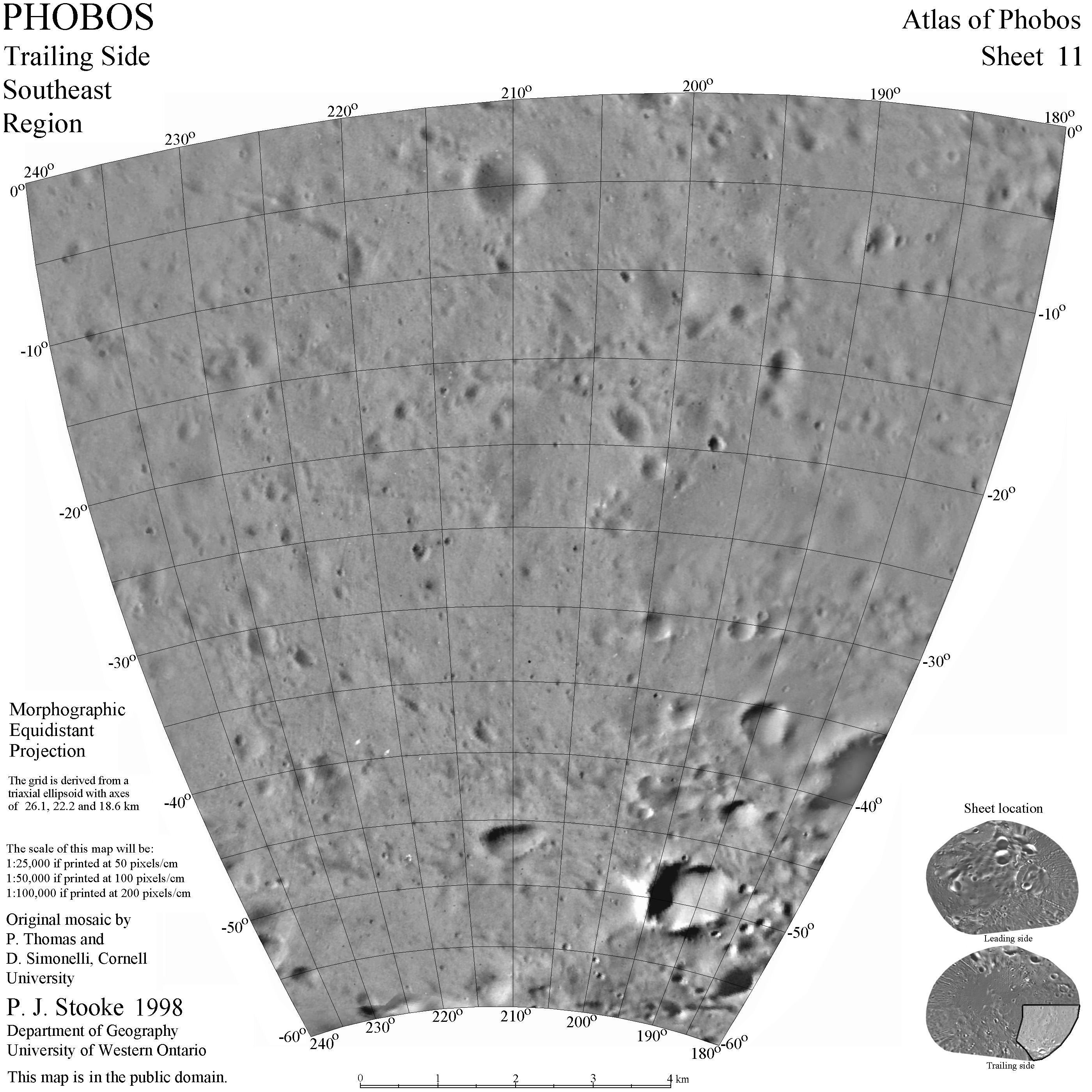
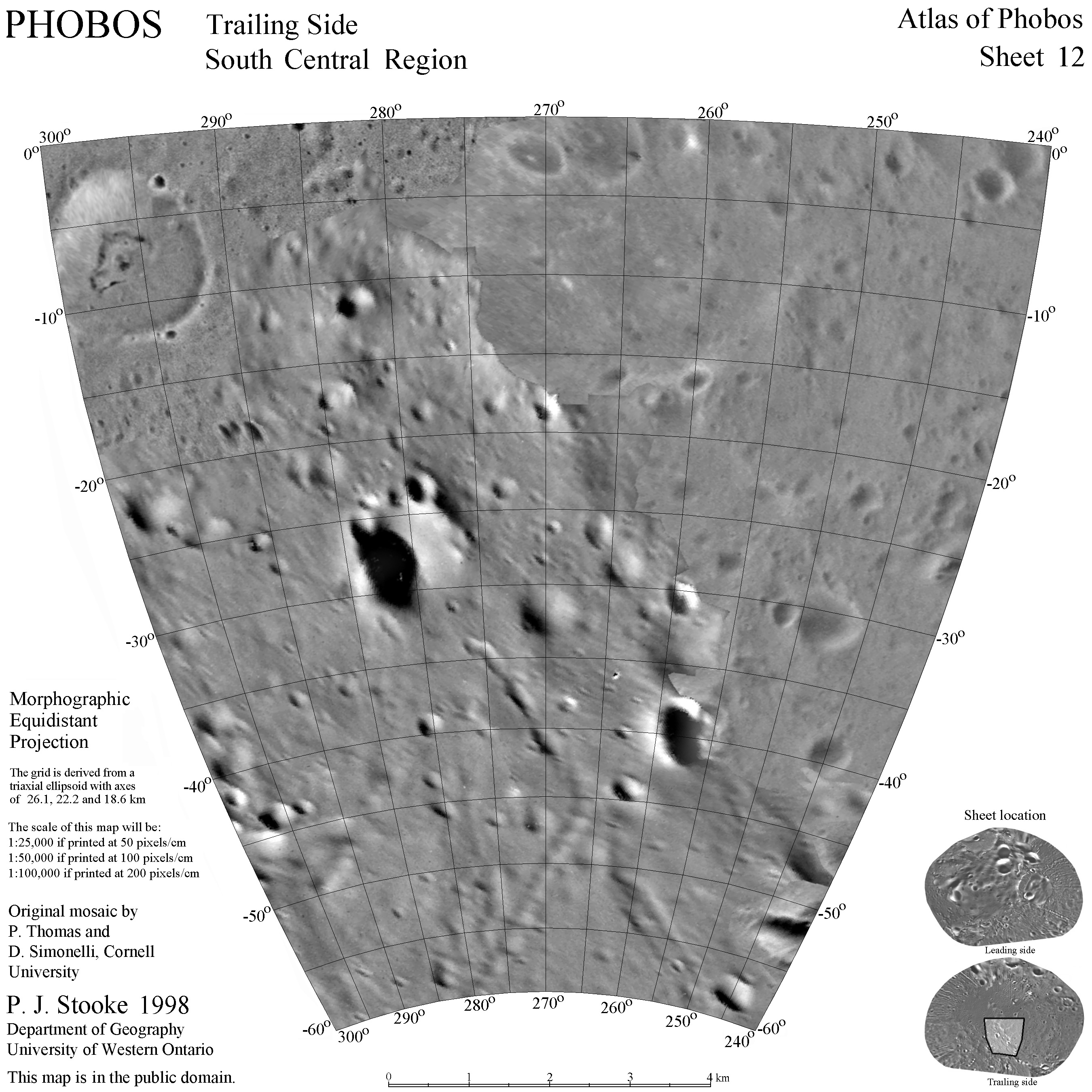
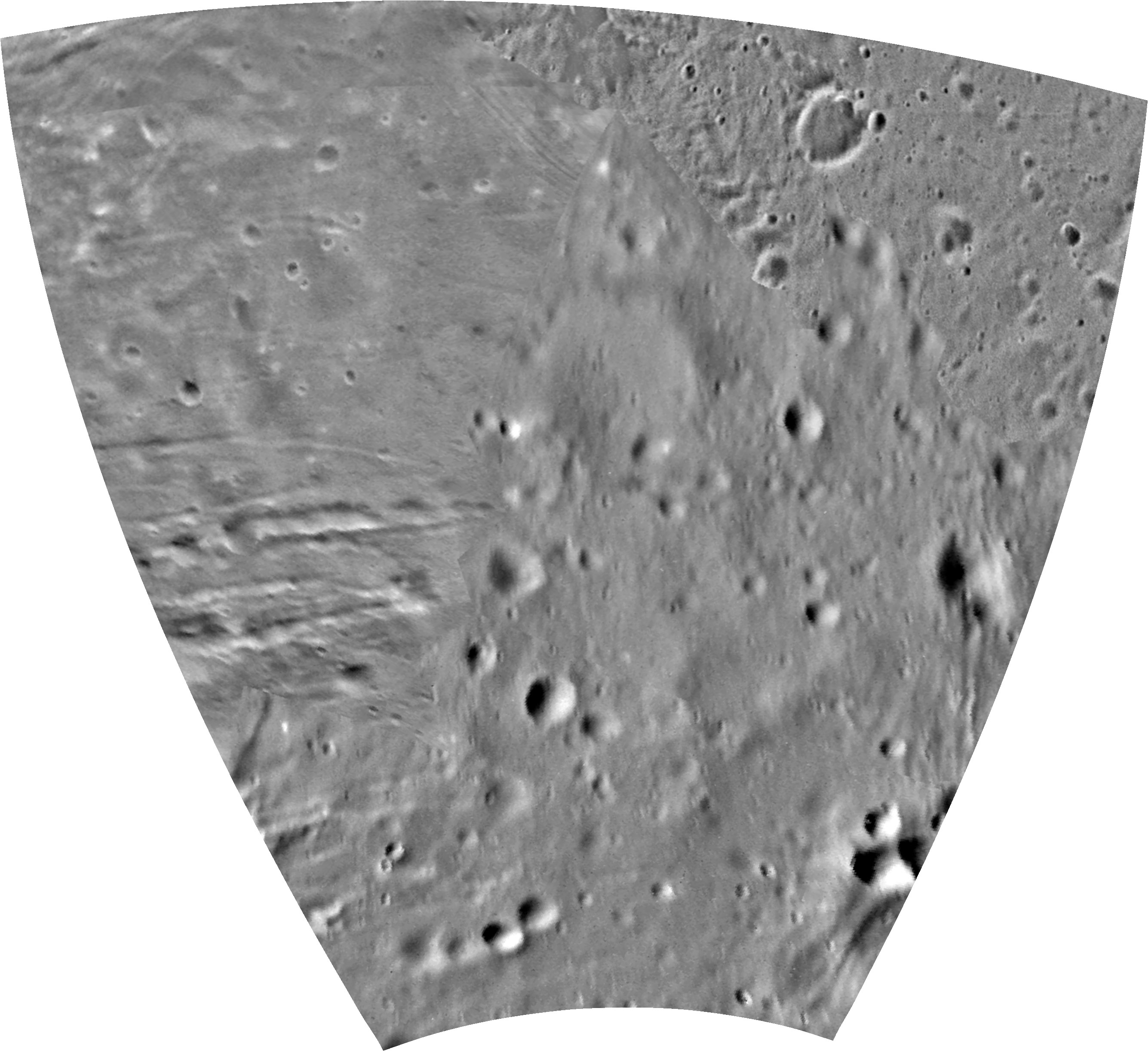
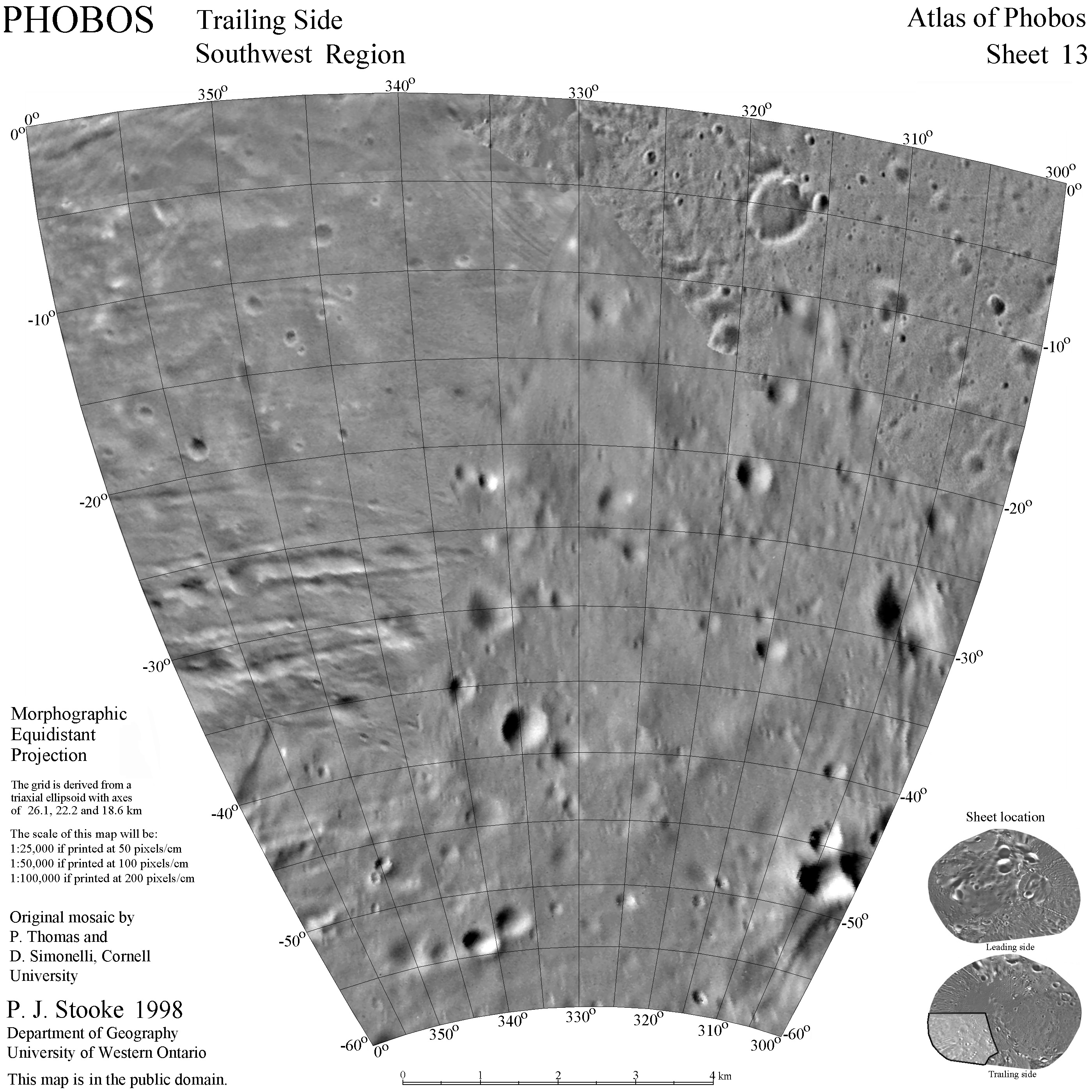
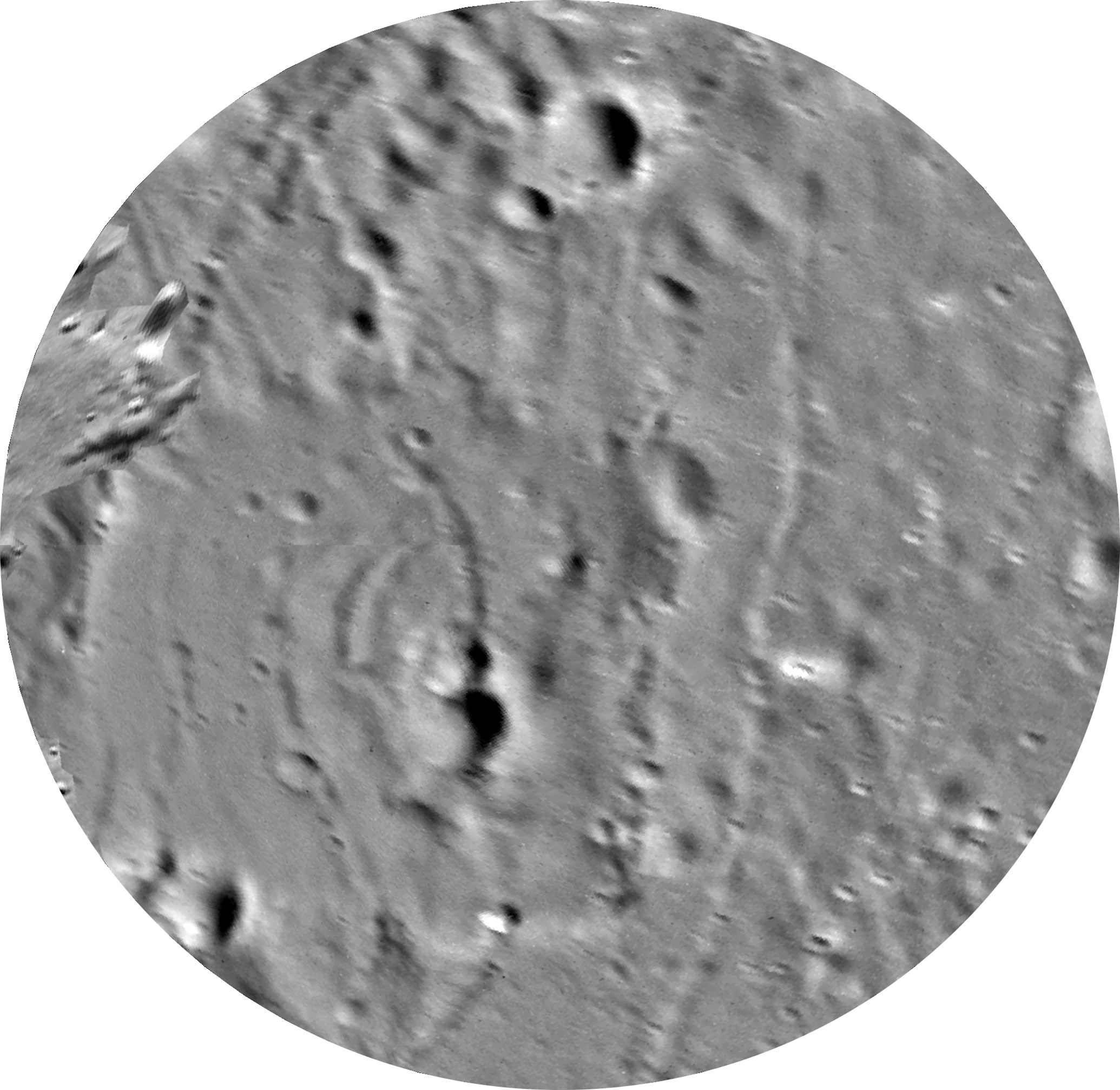
A. Photomosaics from Viking images, in various projections. The mosaics were created initially by Peter Thomas, Damon Simonelli and colleagues at Cornell University, to whom the author is very grateful for permission to use them. They have been modified slightly for this release, then reprojected to a map projection designed for use with non-spherical bodies. The map grids are derived from a best-fit triaxial ellipsoid whose dimensions are given on each map.
These maps cover all of Phobos in 14 sheets, each 60 degrees by 60 degrees,
sheet limits shown on labelled and gridded versions. These maps are superseded
by newly created maps in section E. below.
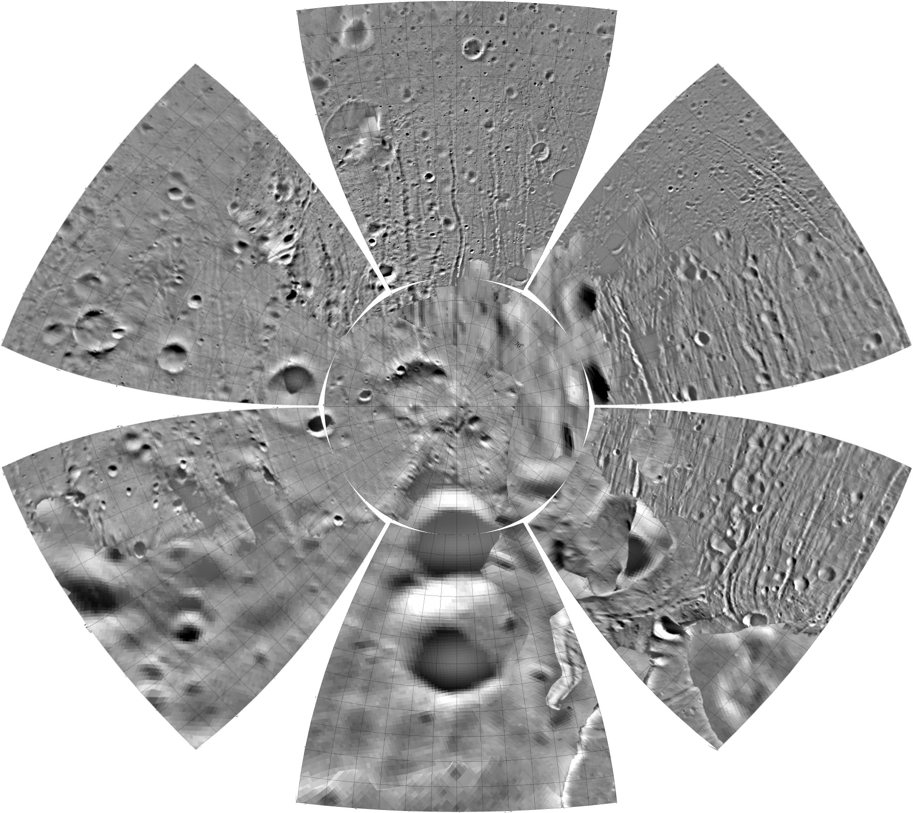
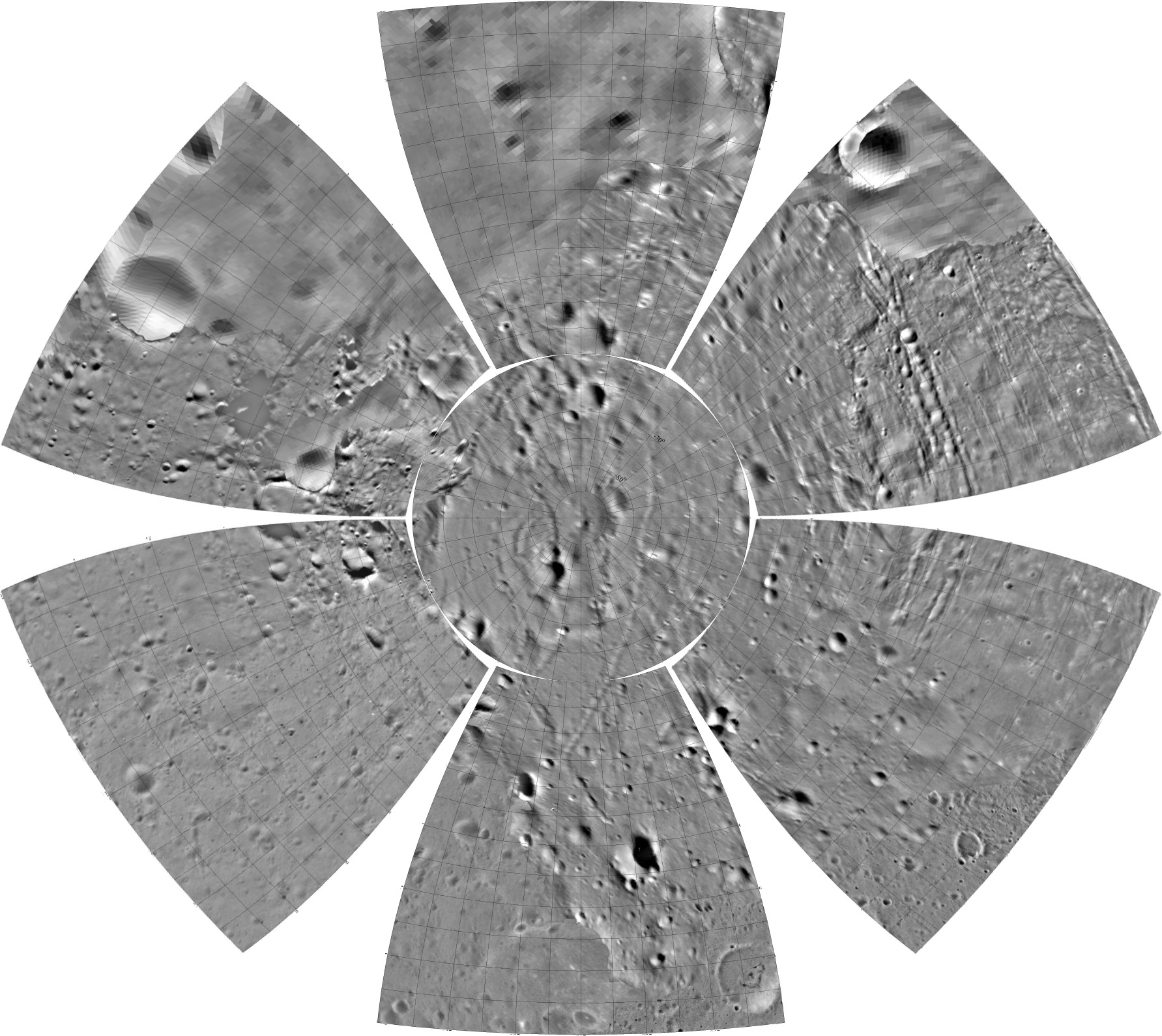
B. Globe gores: Composites of the gridded sheets above arranged around the polar sheets in separate northern and southern hemispheres. These may be cut out and assembled to make a globe, not perfectly shaped but interesting.
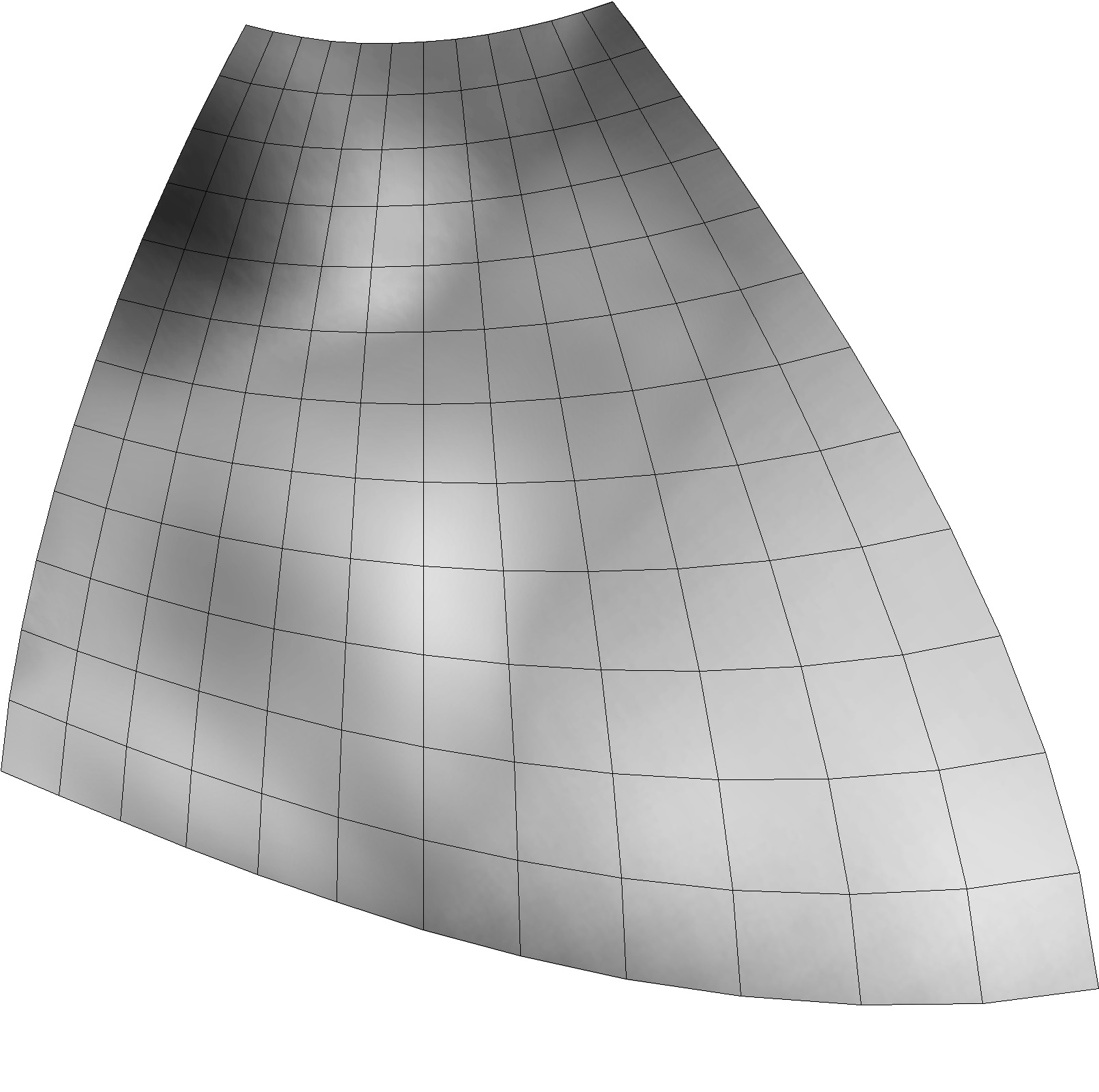
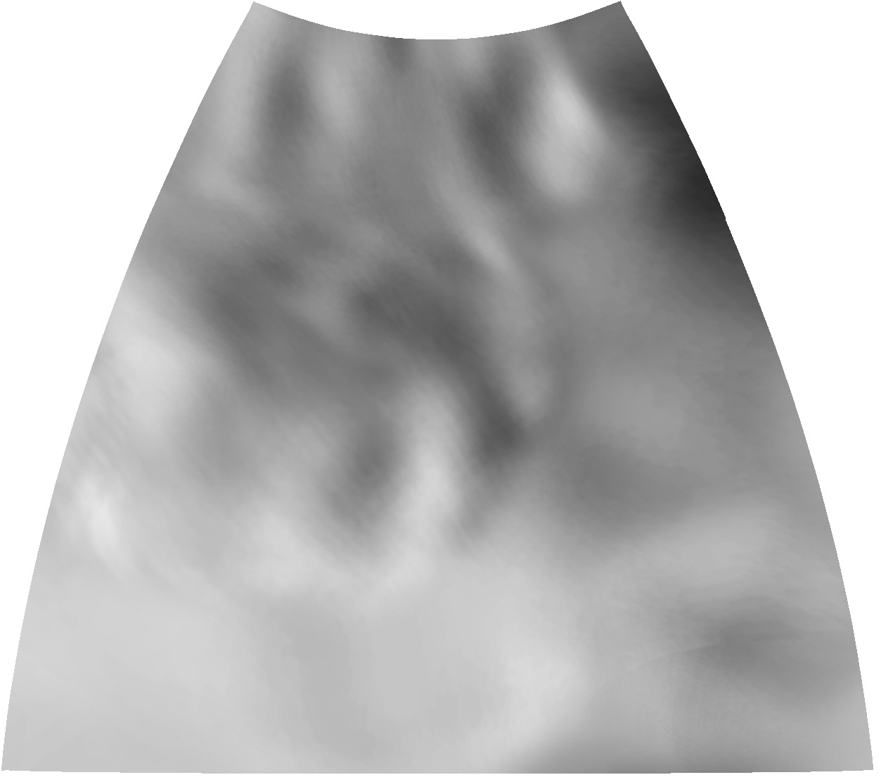
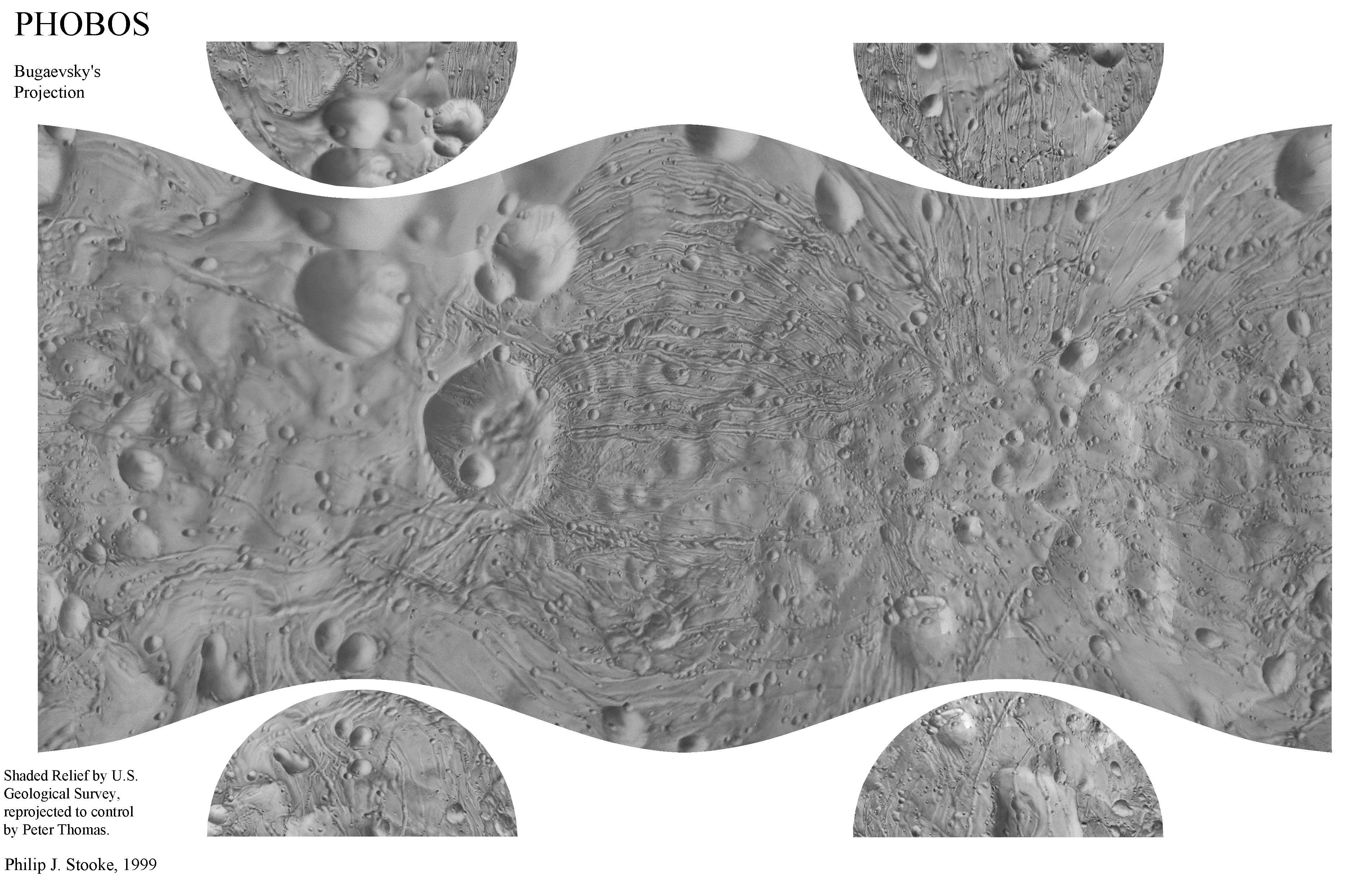
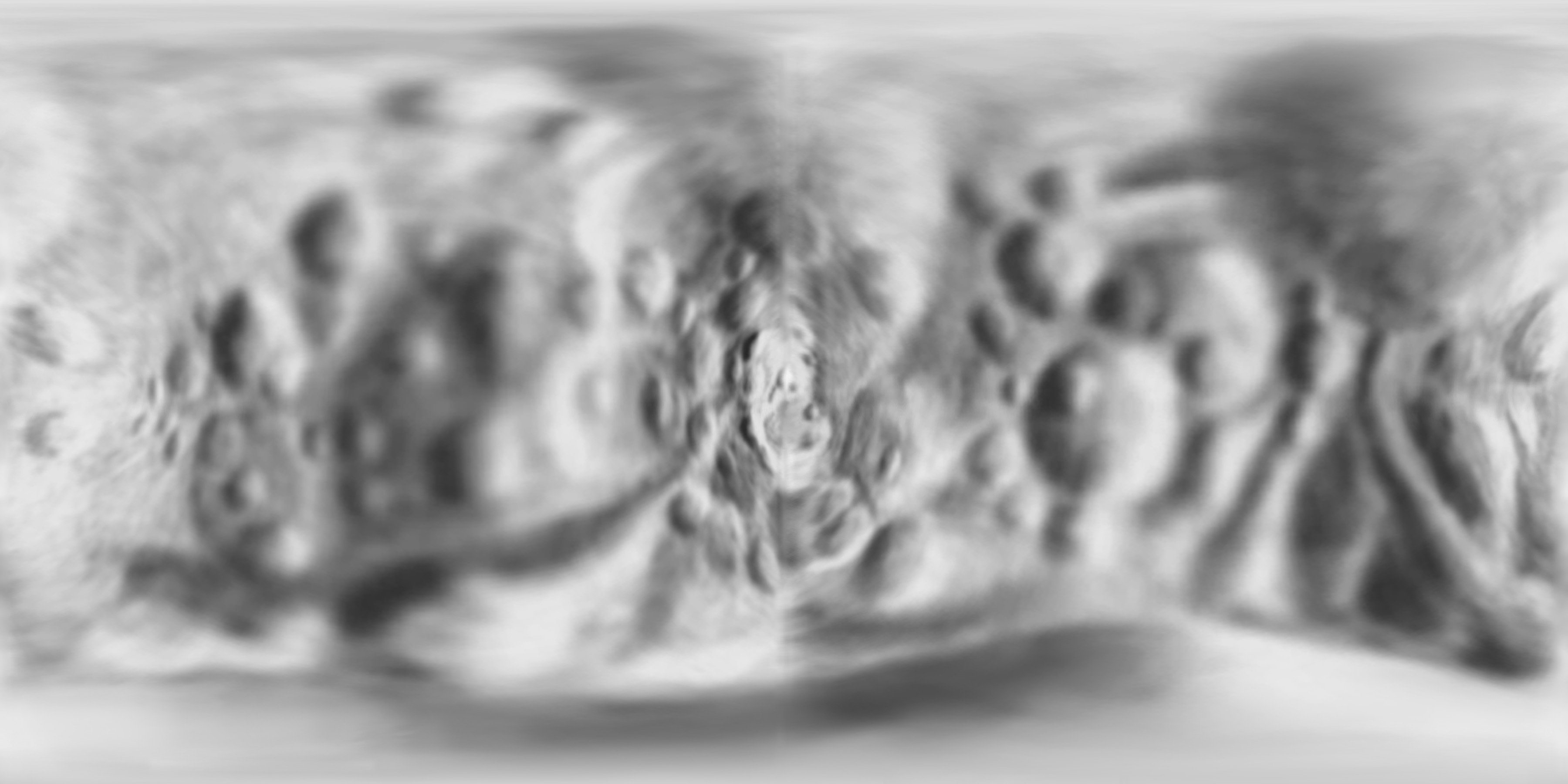
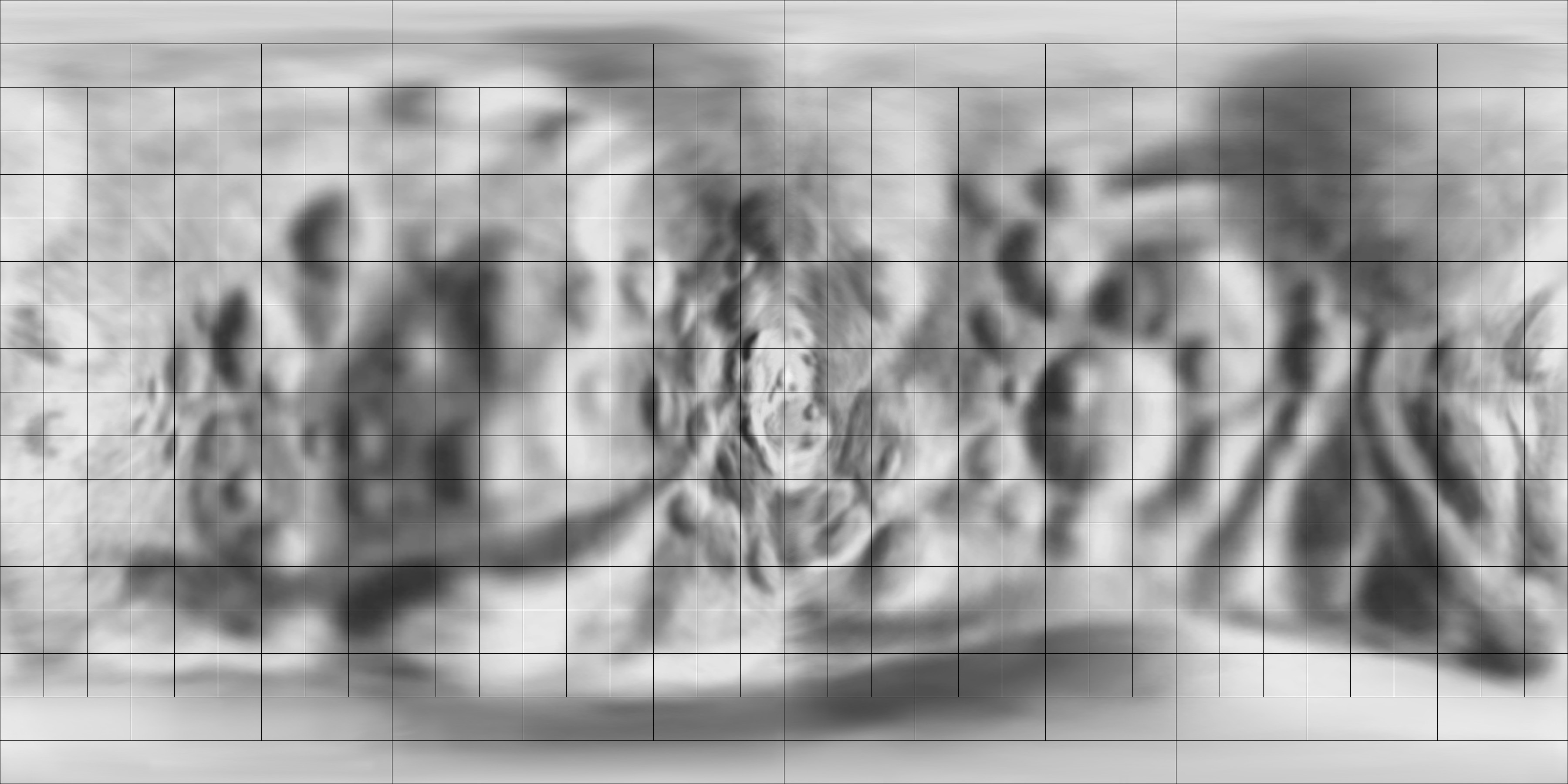
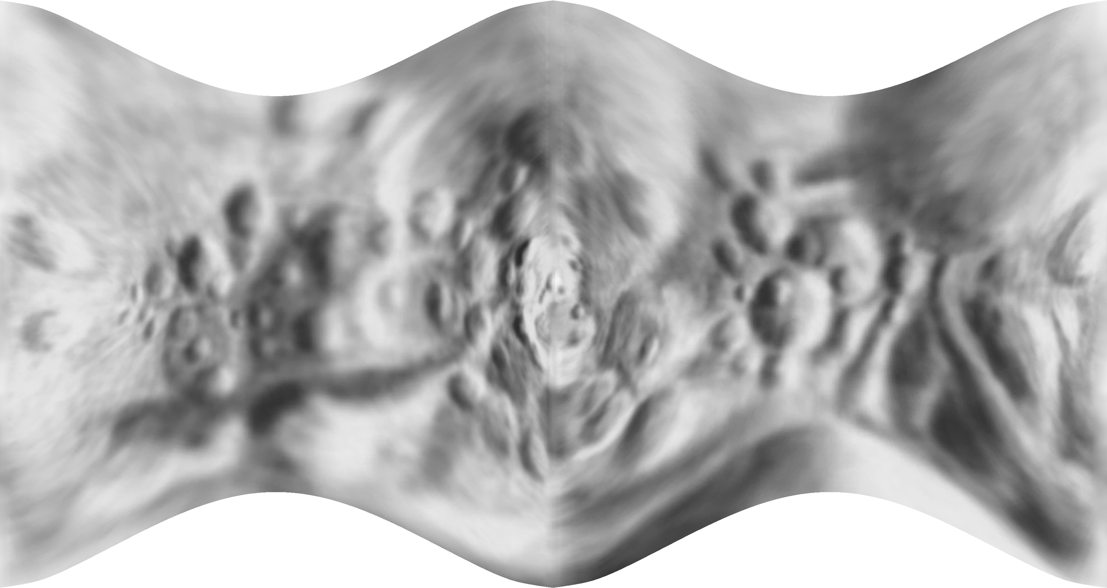
C. Relief maps in various projections.
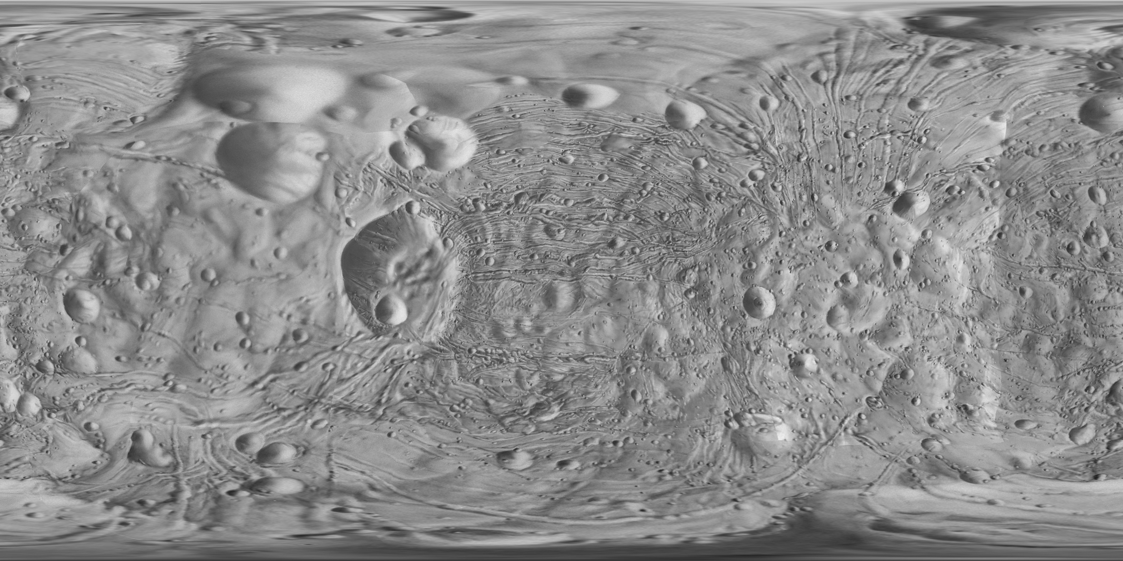
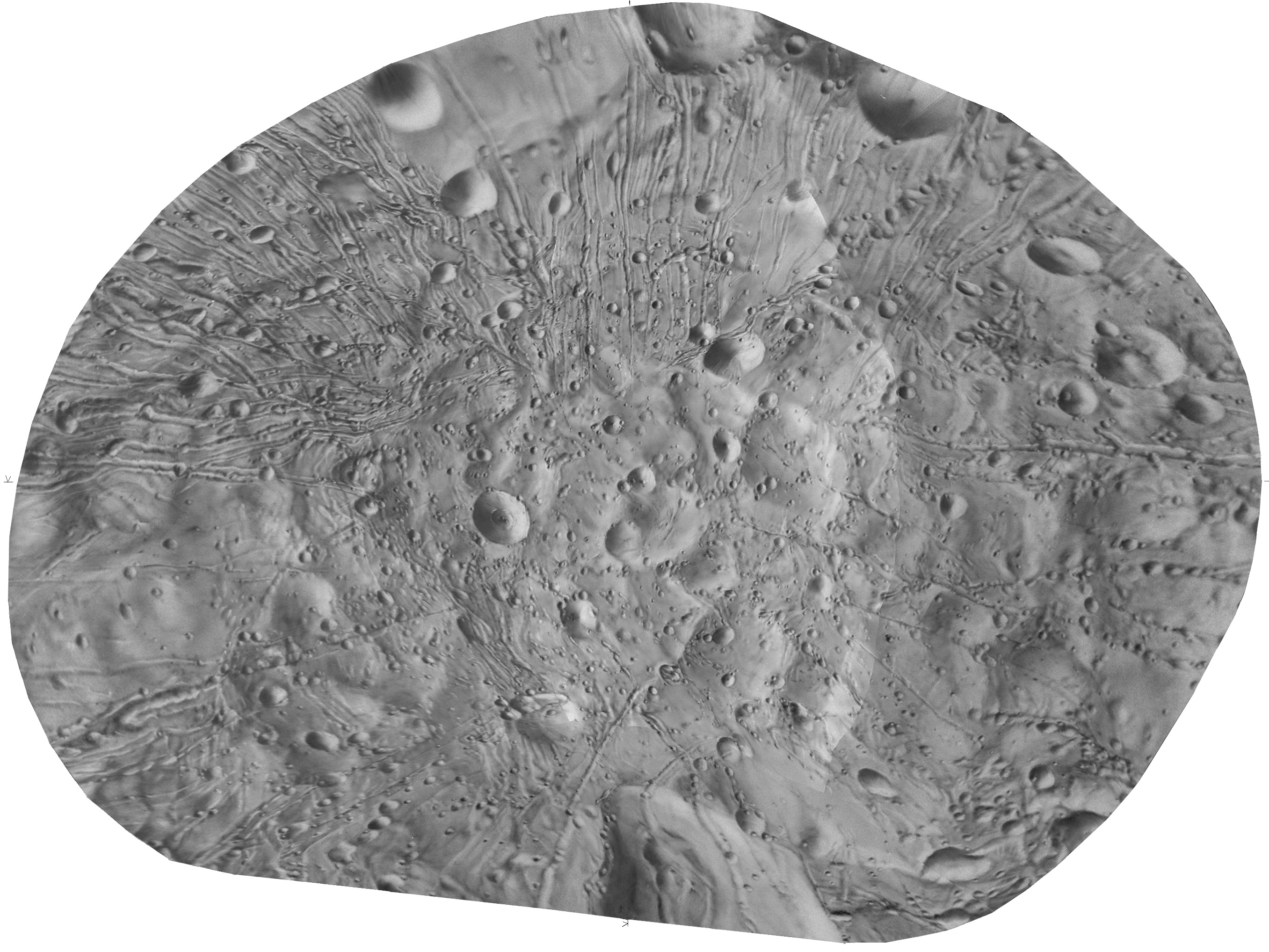
The relief map was created initially by the U. S. Geological Survey. It was based on a shape model considered to be less accurate than that of Thomas and colleagues, and the original contains severe distortions including positional errors of several km, incorrect pole positions and two regions in which surface features were shown twice due to errors in matching images to the shape. For the current version, the relief drawing has been reprojected to fit the control established by Thomas and colleagues, though positional errors of up to one degree (several hundred metres) remain due to limitations of the drawing itself and the reprojection method. It is given here in simple cylindrical projection, polar azimuthal equidistant projection, and in two projections devised specifically for non-spherical worlds: Bugaevsky's conformal cylindrical projection for the triaxial ellipsoid and the Morphographic conformal projection.
D. Global Simple Cylindrical projection mosaics at 10 pixels/degree (3600 by 1800 pixels, 0 longitude at center) of several additional data sets:
Phobos bright markings. This mosaic by P. Stooke and S. Berry, based on positional control by P. Thomas, is constructed from low phase angle images by the Viking Orbiters and Phobos 2. It is designed to show only the locations of local bright markings on Phobos, not the true albedo. Some bright markings may be caused by local photometric function variations (caused by variations in grains size, etc.) rather than true albedo variations. Photometric validity was intentionally sacrificed during image processing.
Bright markings superimposed on Viking photomosaic. The previous file superimposed on the Viking Orbiter mosaic of Peter Thomas, intended to show the relationship between bright markings and local topography.
Viking image mosaic with lat/lon grid. Mosaic by Peter Thomas, overlaid with an unlabelled grid at ten degree spacing.
Mariner 9 photomosaic by P. Stooke and J. Pfau, University of Western Ontario.
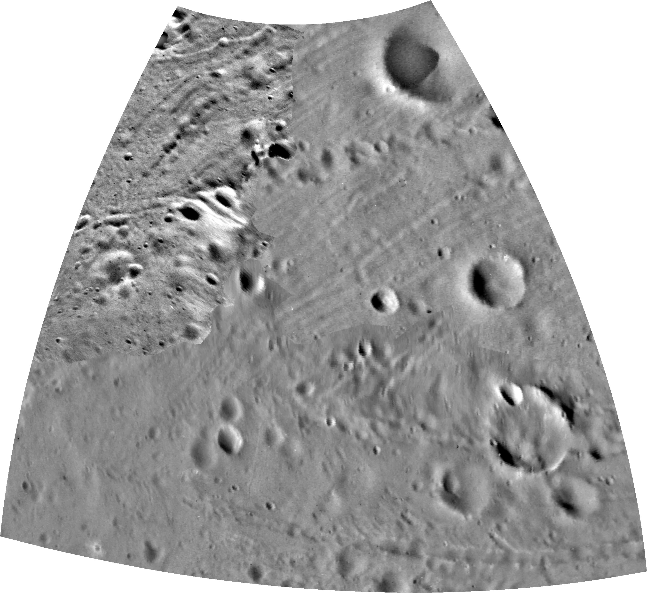
E. Cornell Control and DLR Control improved photomosaics
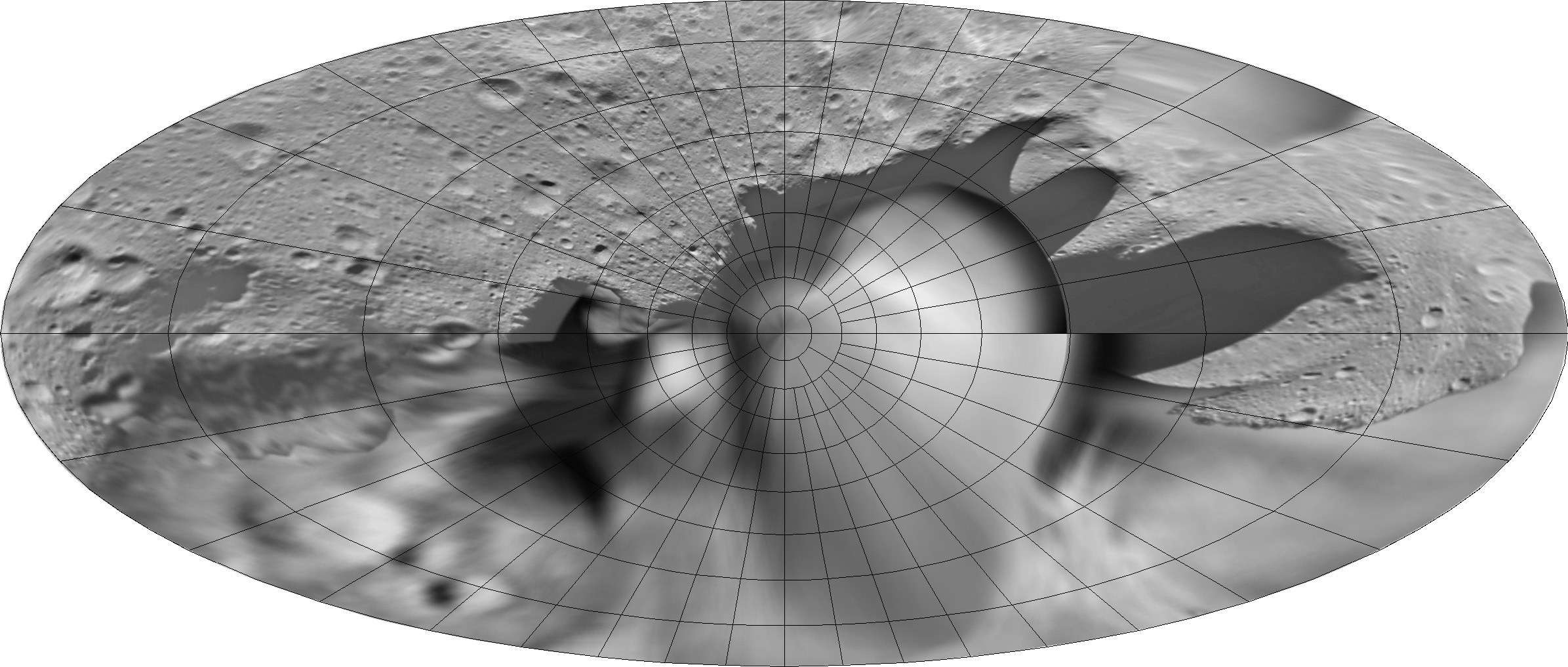
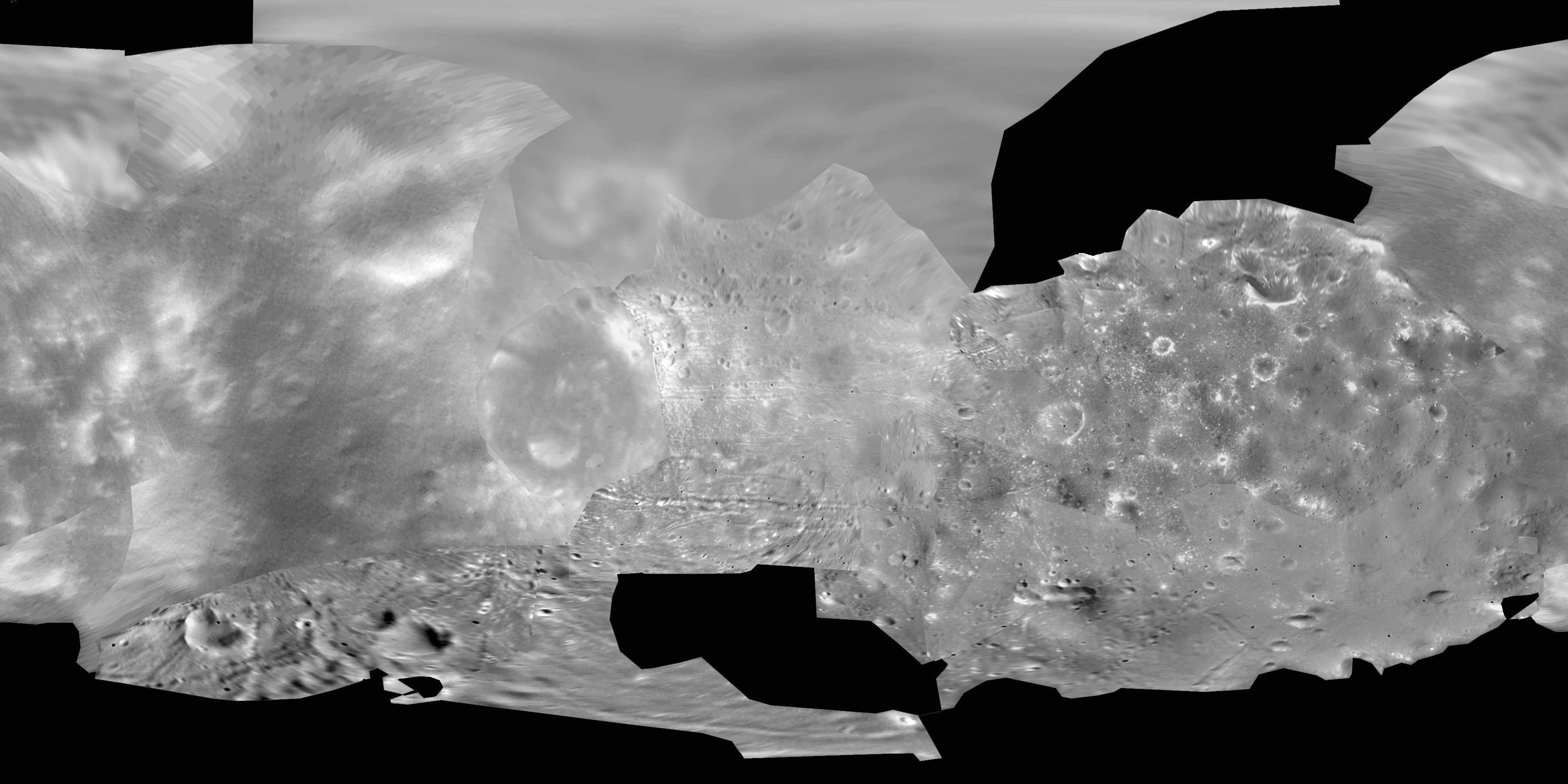
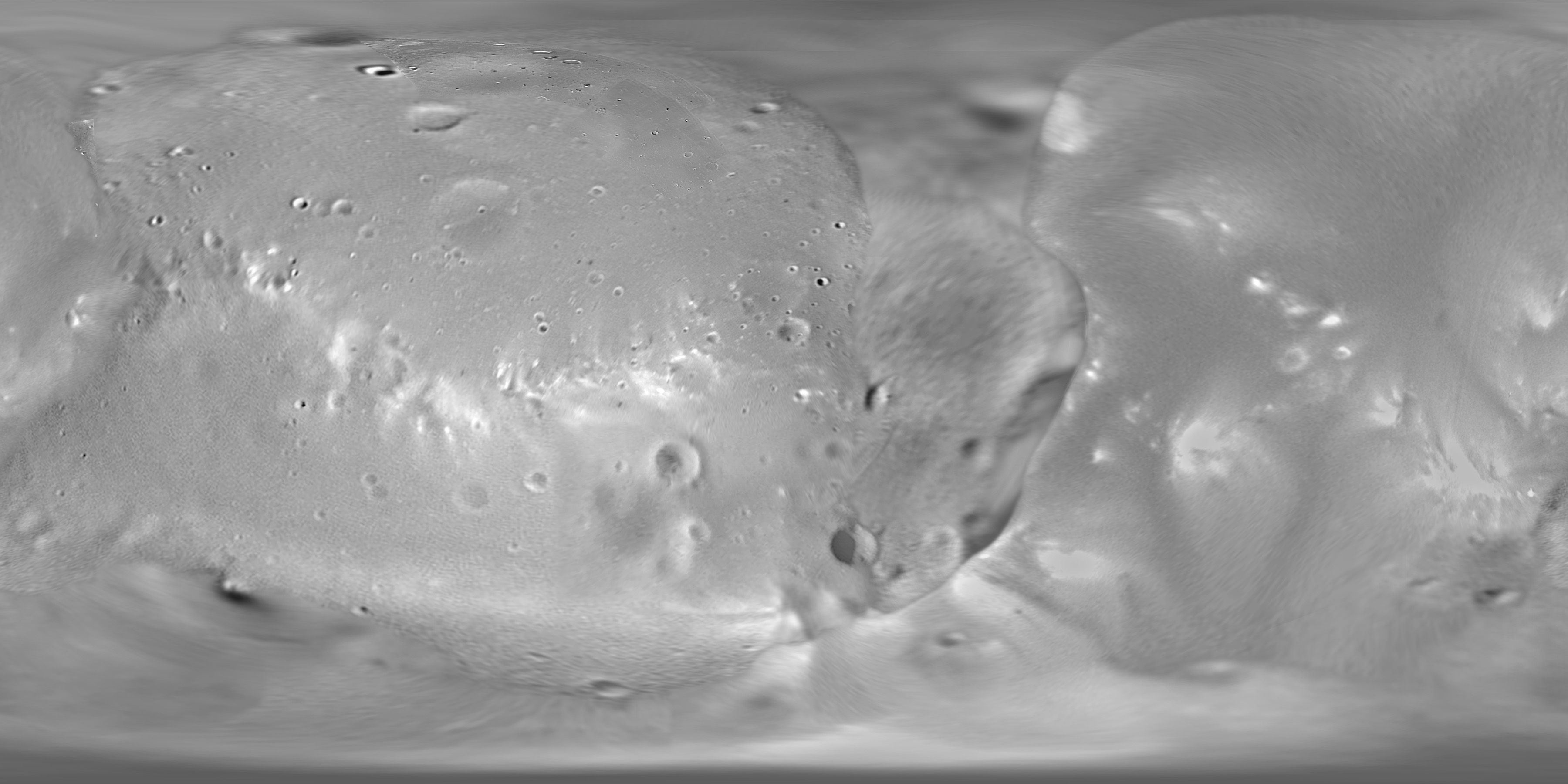
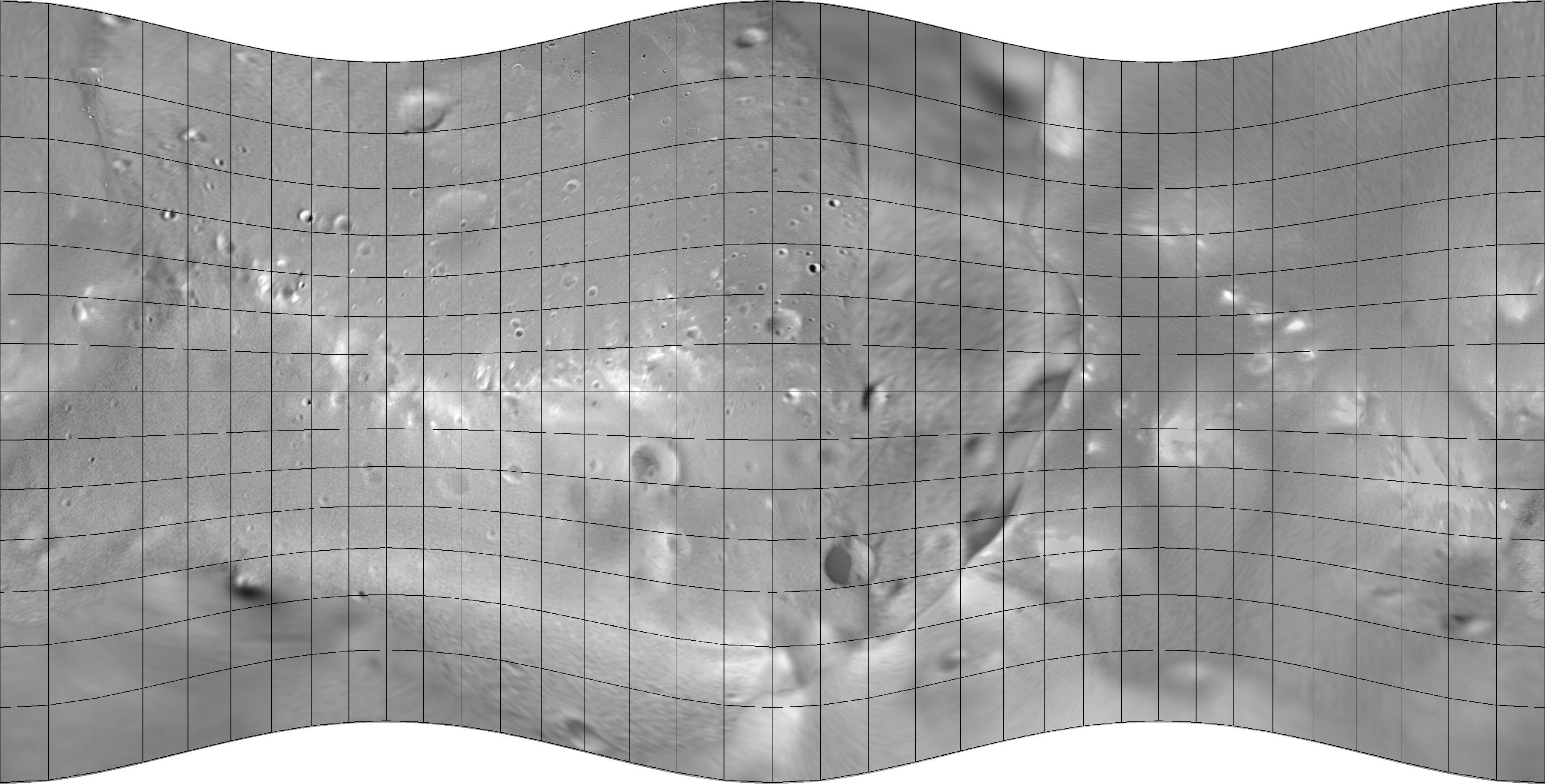
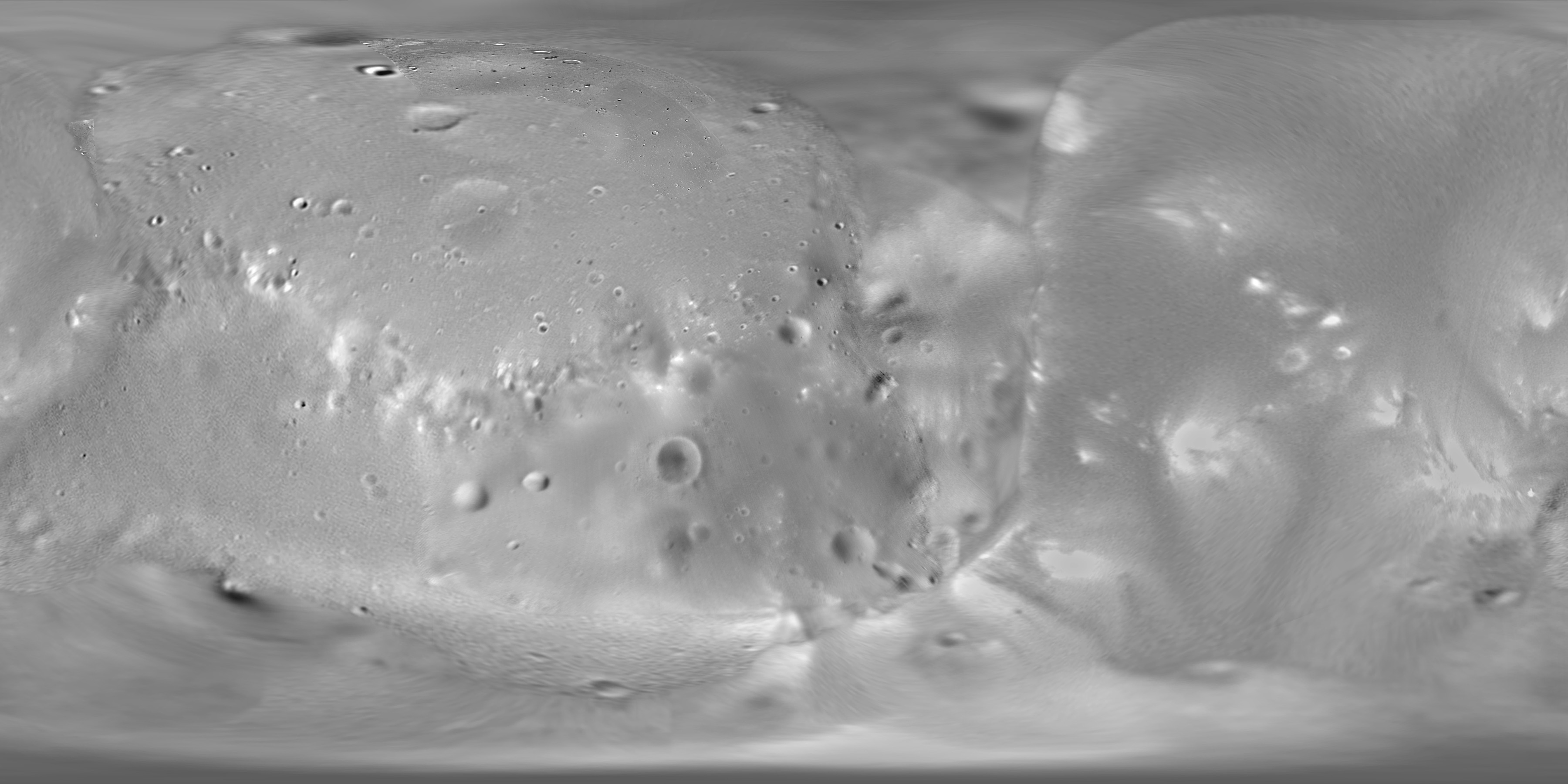
The best previous Phobos map was the global photomosaic compiled at Cornell University by Simonelli et al. (1993), listed above in section A. That mosaic consisted of Viking Orbiter images. Since it was made, numerous additional images have been taken by Mars Global Surveyor, Mars Express and Mars Reconnaisance Orbiter. Many of these are superior to Viking images in resolution, especially in the region west of Stickney that was least well seen by Viking. This new mosaic was created by compiling new versions of the original Viking high resolution mosaics, and selecting the best high resolution images from the other spacecraft, so that an entirely new mosaic could be constructed. Control was provided by the Cornell mosaic. In the process of compiling the mosaic, some areas poorly controlled in the old mosaic were significantly improved (e.g. near 40 north, 140 east longitude, where only very oblique Viking images were available but Mars Express provides a near-vertical view). The Cornell mosaic was enlarged to 14400 by 7200 pixels to accommodate higher resolution images. In each area the best available images were reprojected and combined. Where images with reverse lighting meet, artistic effects are necessary to create a satisfactory appearance, but this affects only the appearance and not the map geometry.
Simple Cylindrical Projection , north at the top, 0 longitude at the center, 14400 by 7200 pixels. (40 pixels/degree)
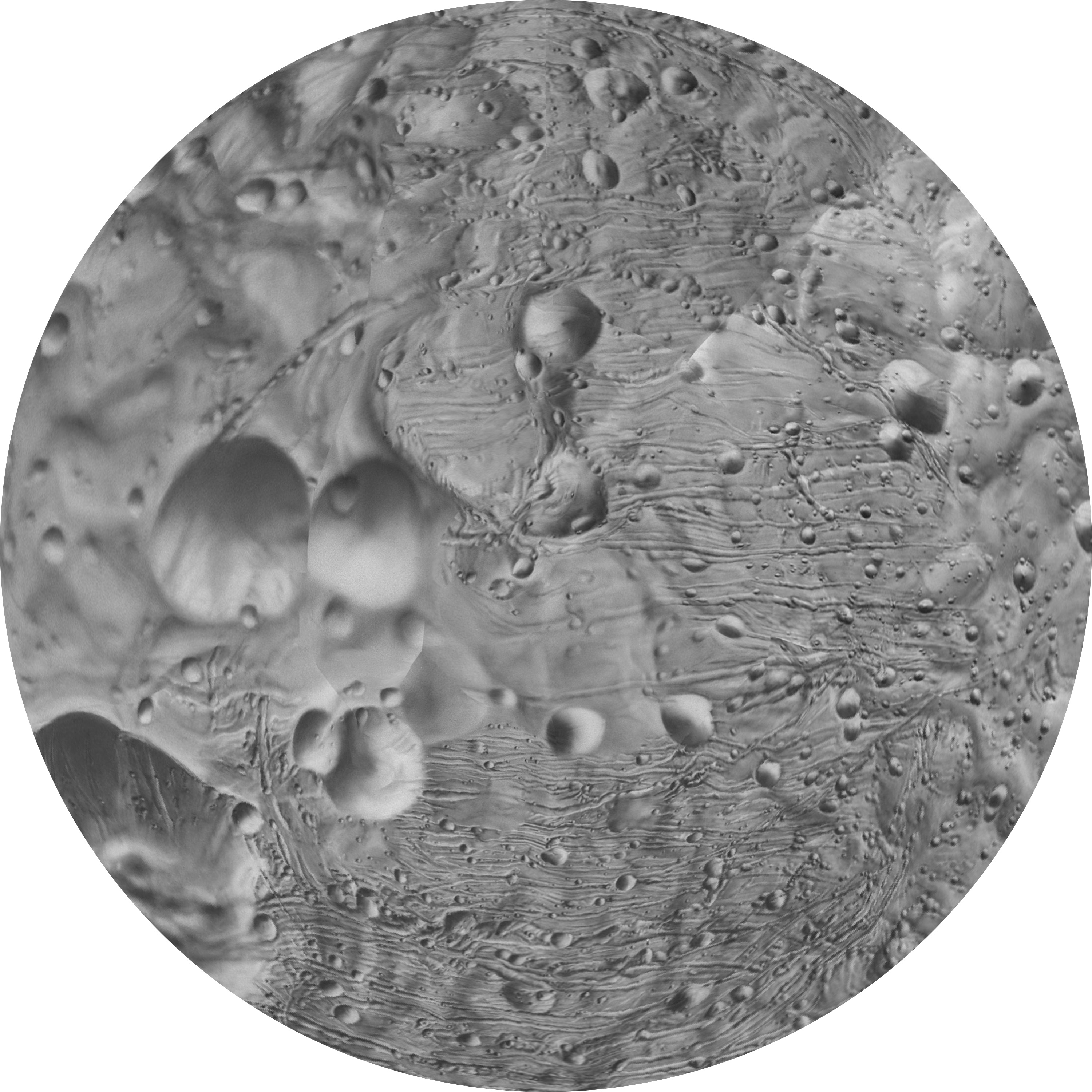
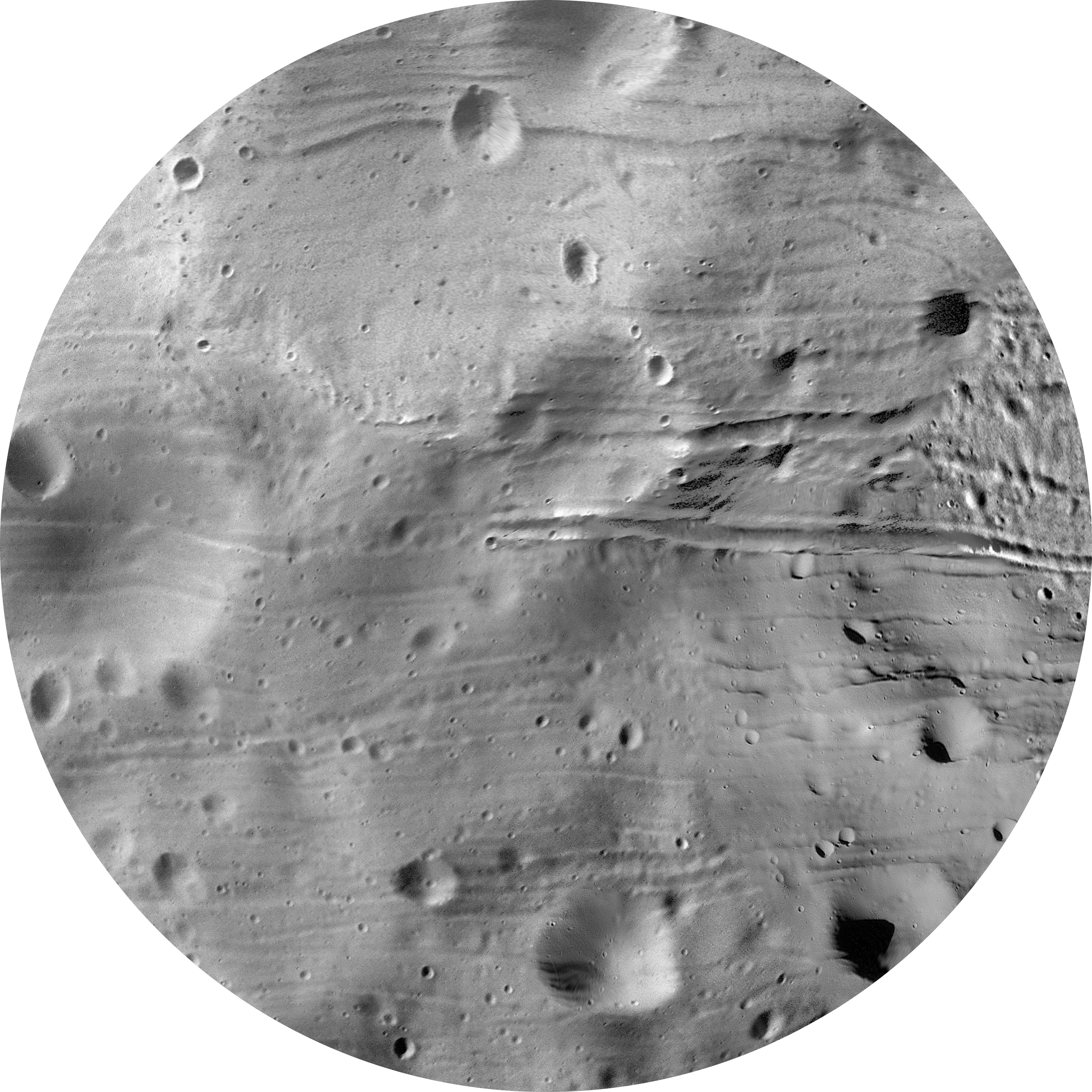
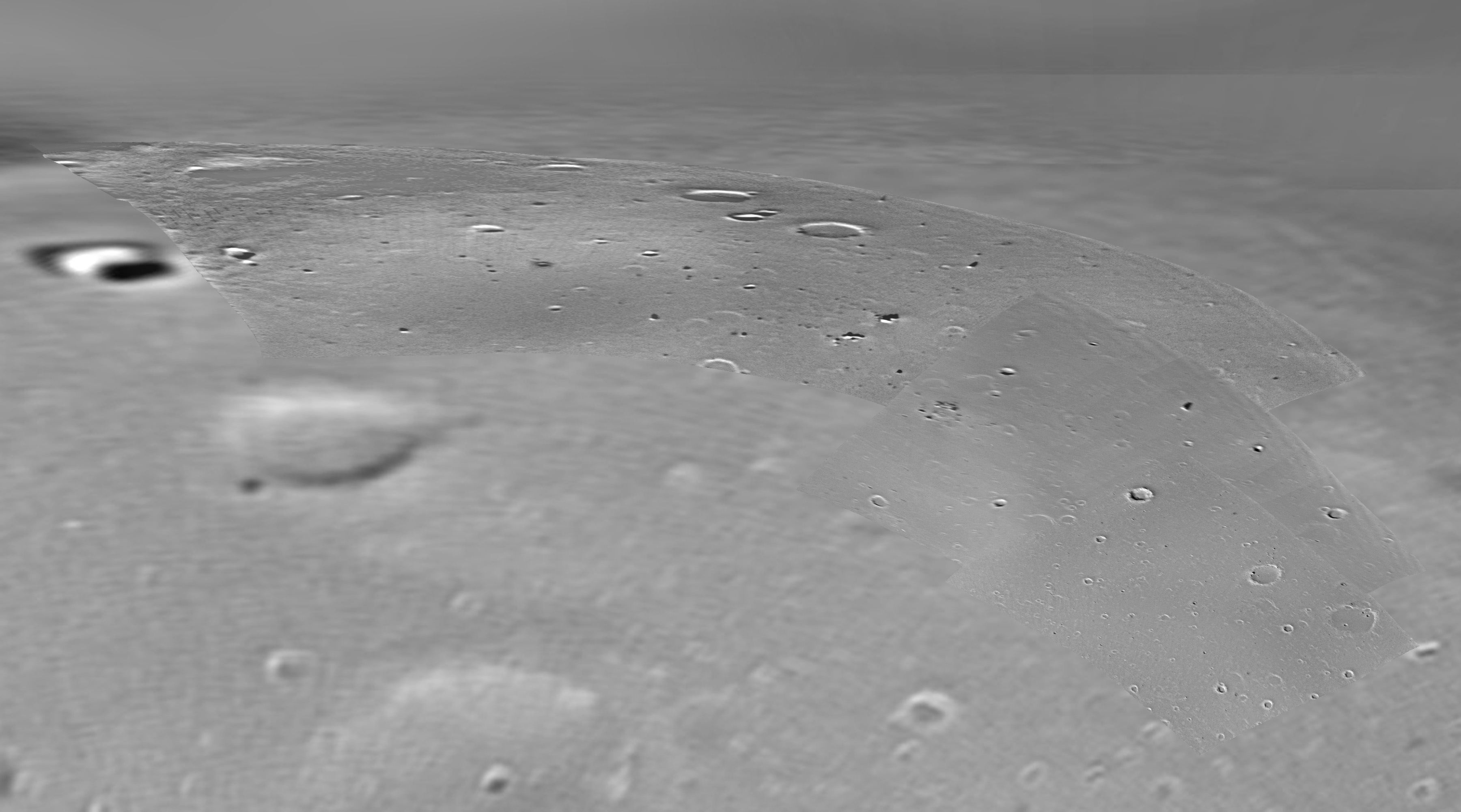
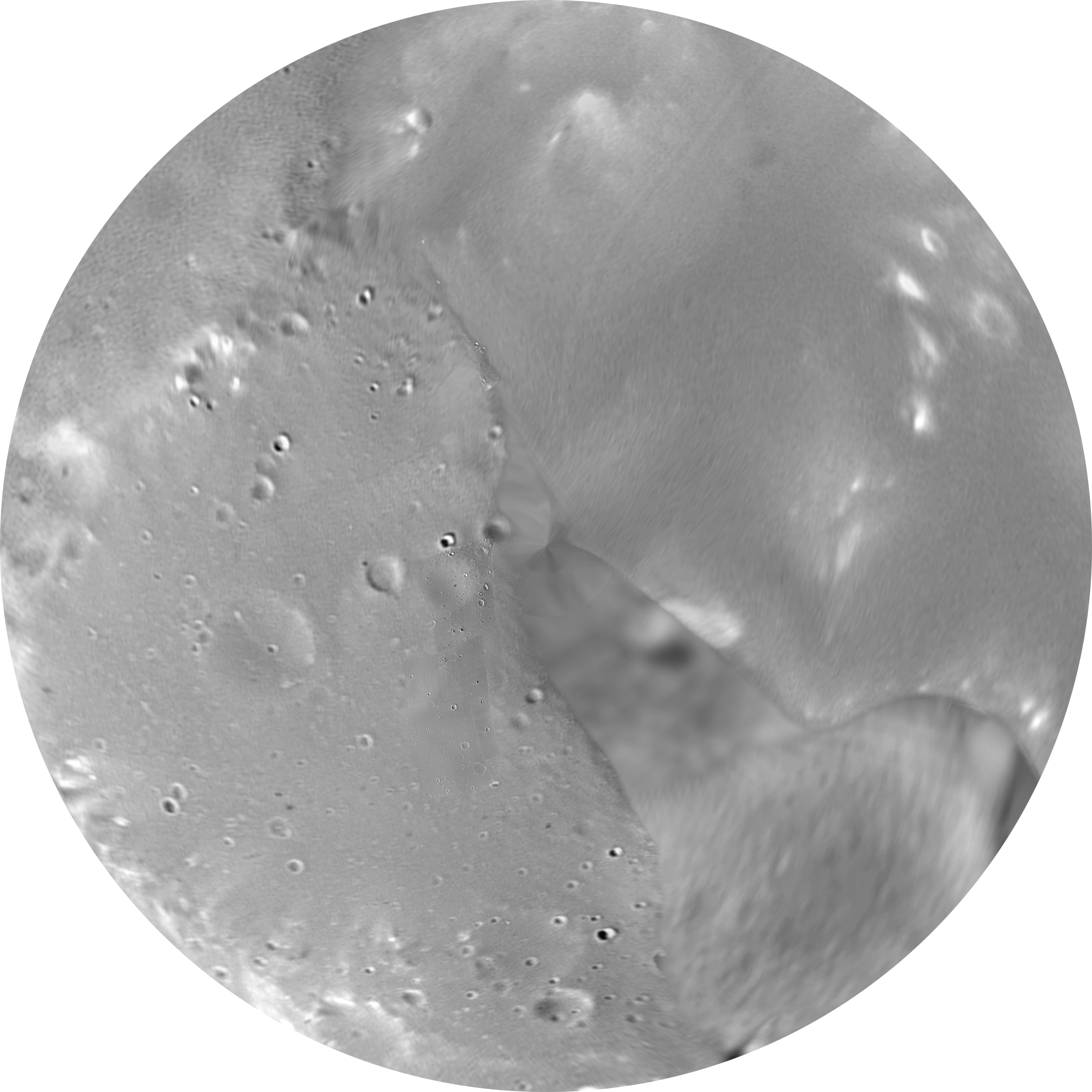
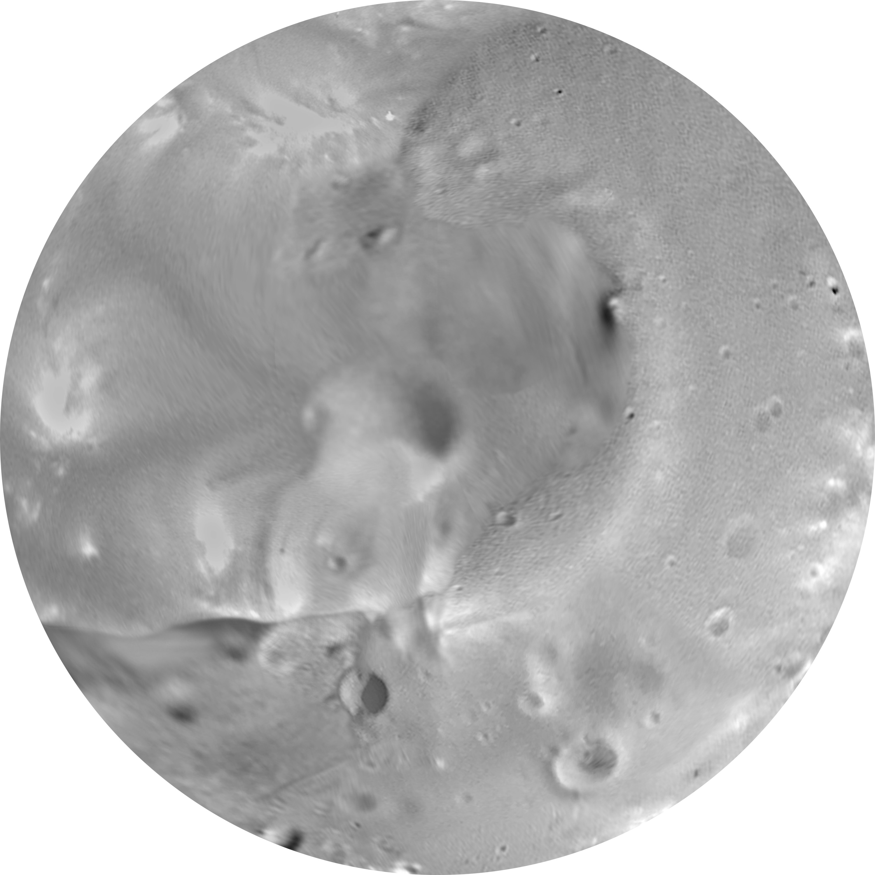
Polar Equidistant Projection North (latitudes equally spaced), 0 longitude at the top, north pole at center, 50 degrees north at the outer edge.
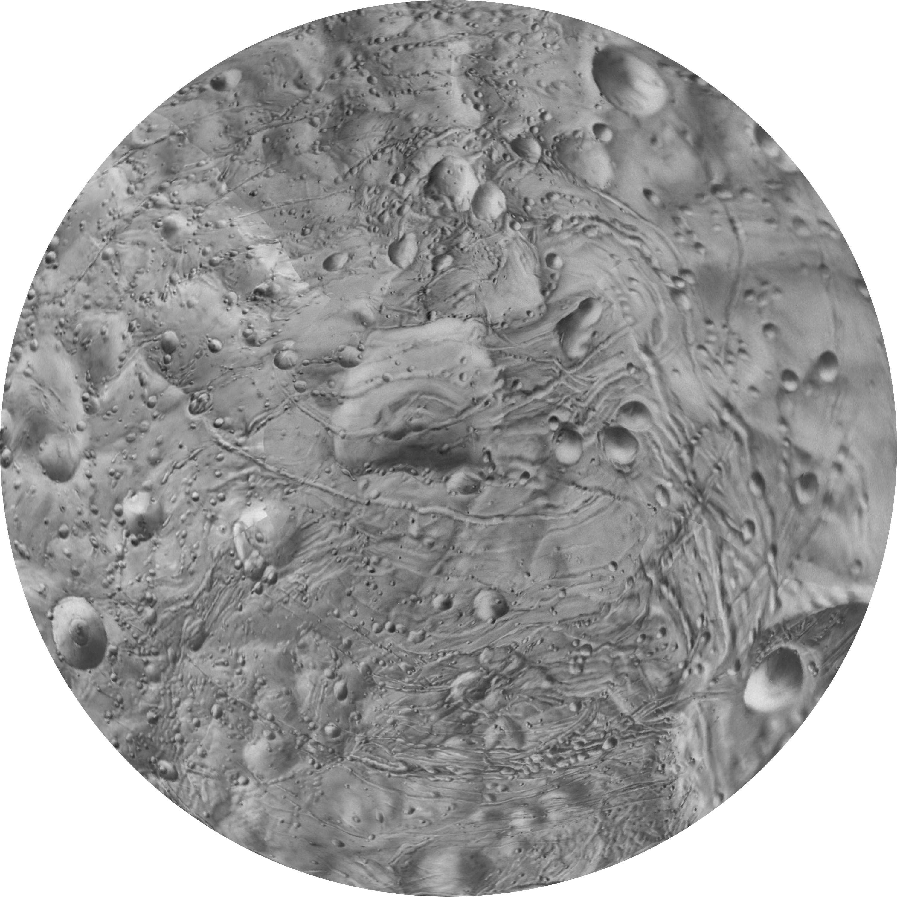
Polar Equidistant Projection South (latitudes equally spaced), 0 longitude at the top, south pole at center, 50 degrees south at the outer edge.
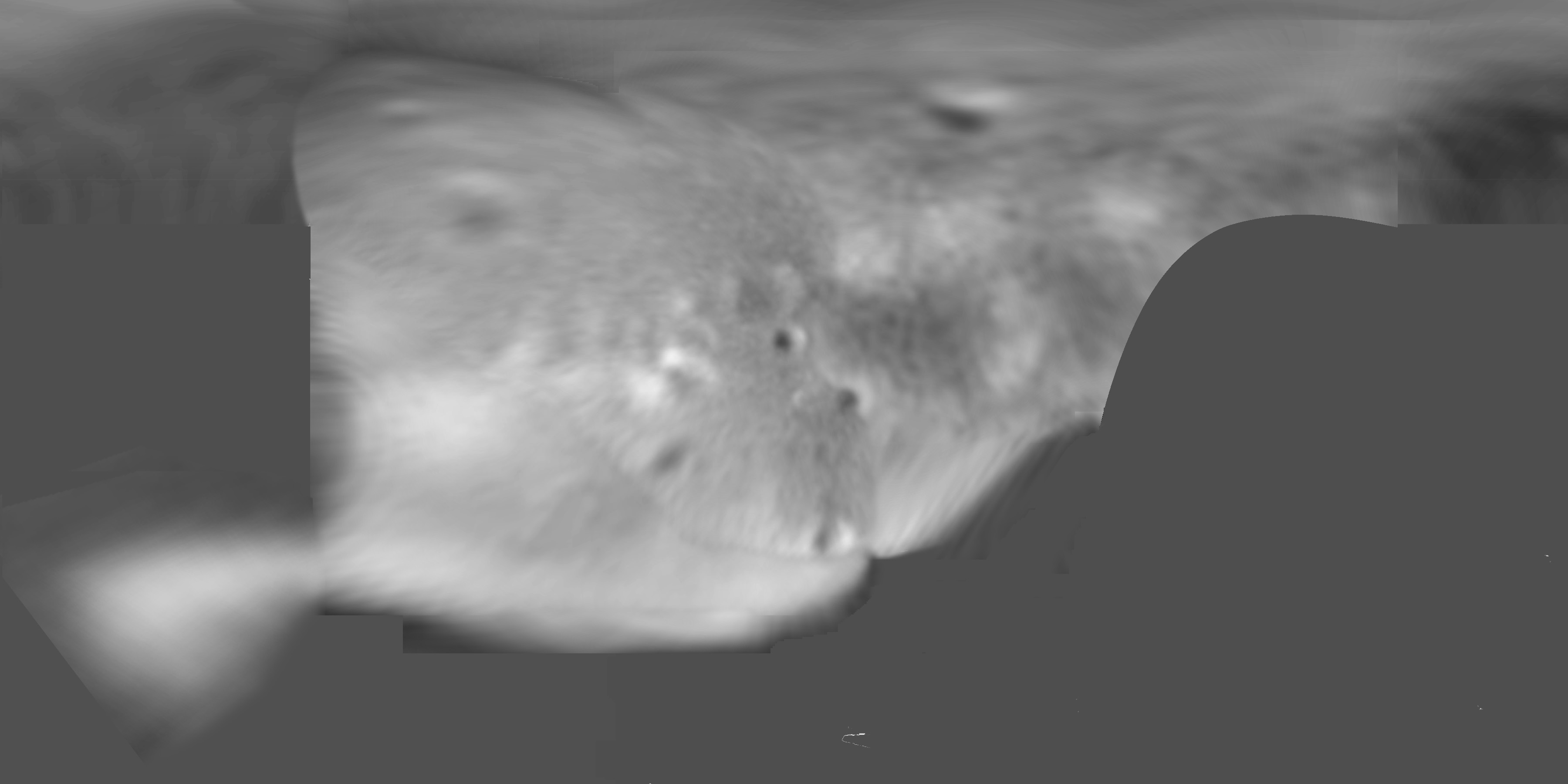
A second map of Phobos was created to match the new control from DLR described by Waehlisch et al. (2009) and Willner et al. (2010). The mosaic based on Cornell control was reprojected to match the DLR control. Low resolution, image gaps and some bad seams in the original DLR mosaic make this reprojection only an approximate match to the DLR geometry. It is the best that can be done at present. Both versions of the Phobos mosaic are presented here so that visualizations based on either shape model can incorporate the appropriate mosaic.
Simple Cylindrical Projection , north at the top, 0 longitude at the center, 14400 by 7200 pixels. (40 pixels/degree)
Polar Equidistant Projection North (latitudes equally spaced), 0 longitude at the top, north pole at center, 50 degrees north at the outer edge.
Polar Equidistant Projection South (latitudes equally spaced), 0 longitude at the top, south pole at center, 50 degrees south at the outer edge.
References:
Simonelli, D.P., P.C. Thomas, B.T. Carcich, and J. Veverka, The generation and use of numerical shape models for irregular solar system objects, Icarus 103, 49-61, 1993.
Waehlisch, M. et al., A new topographic image atlas of Phobos, Earth Planet. Sci. Lett., doi:10.1016/j.epsl.2009.11.003, 2009. (Available online at http://europlanet.dlr.de/node/index.php?id=214.)
Willner, K., Oberst, J., Hussmann, H., Giese, B., Hoffmann, H., Matz, K., Roatsch, T., and Duxbury, T.: Phobos control point network, rotation, and shape, Earth and Planetary Science Letters, Vol. 294 (3-4), pp.547-553, 2010.
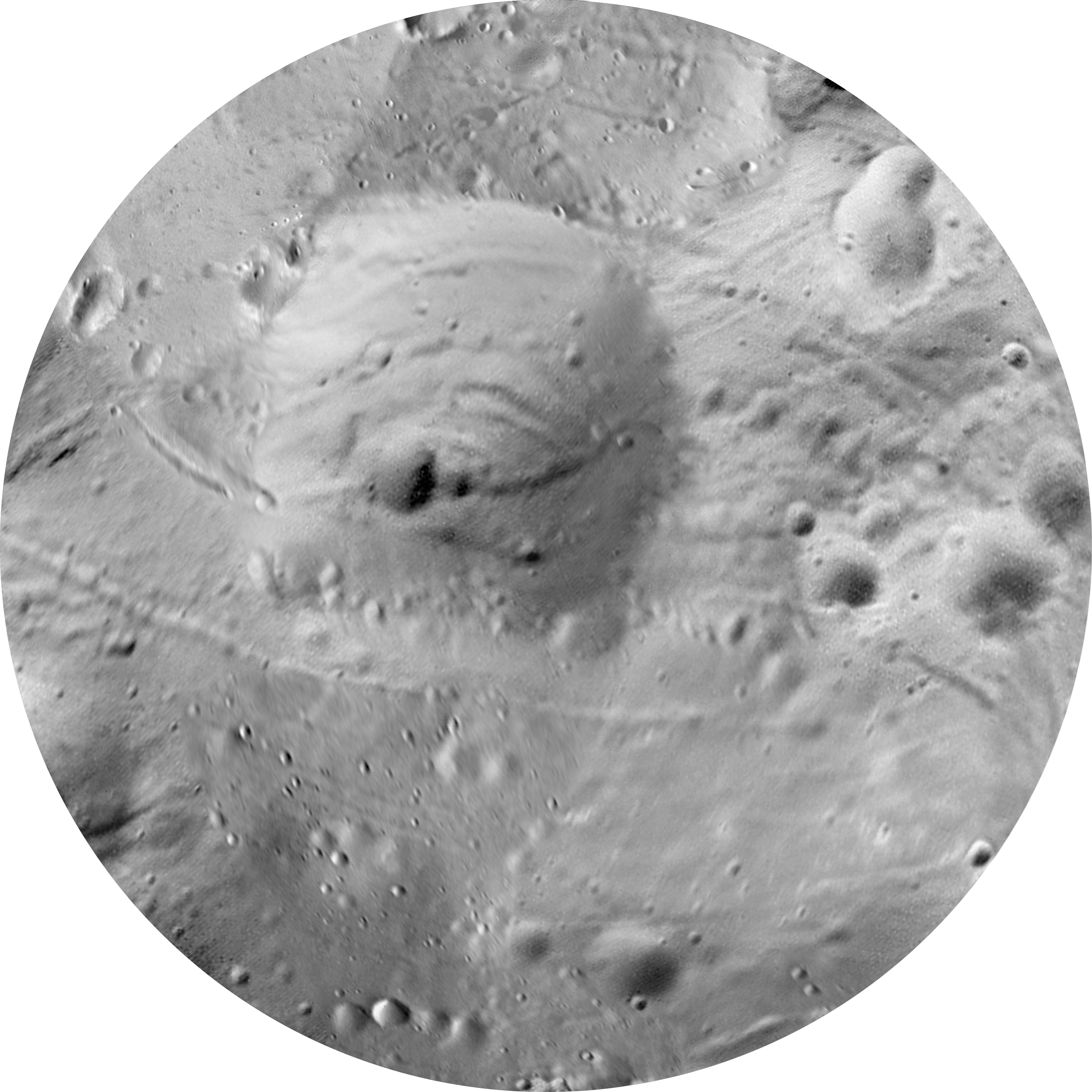
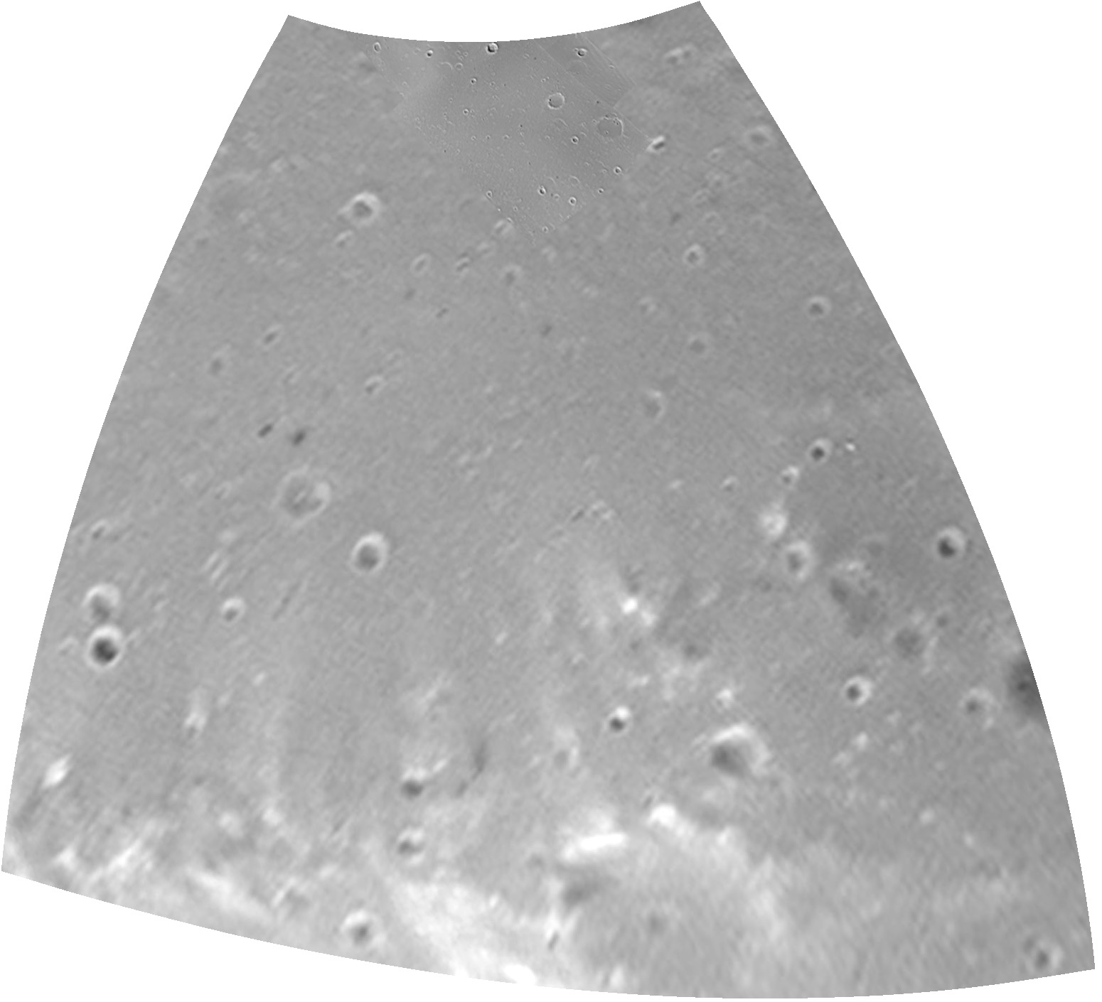
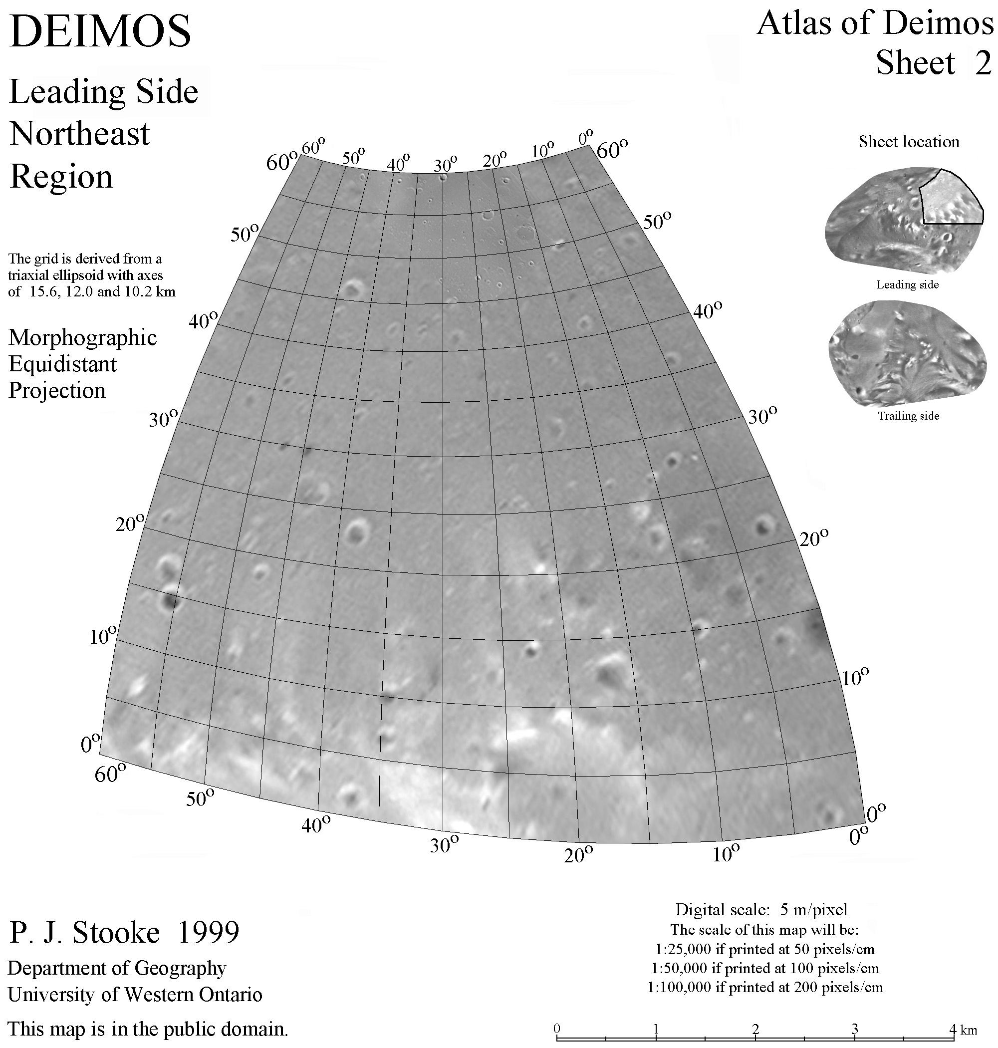
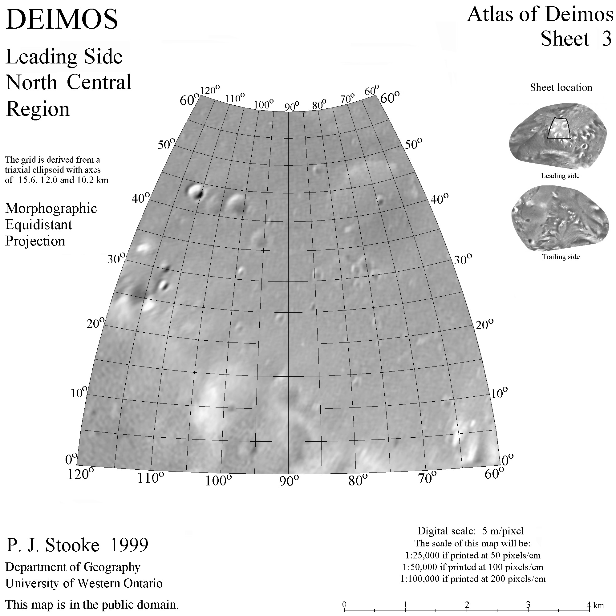
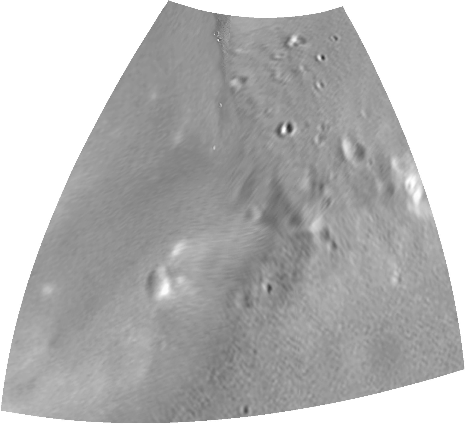
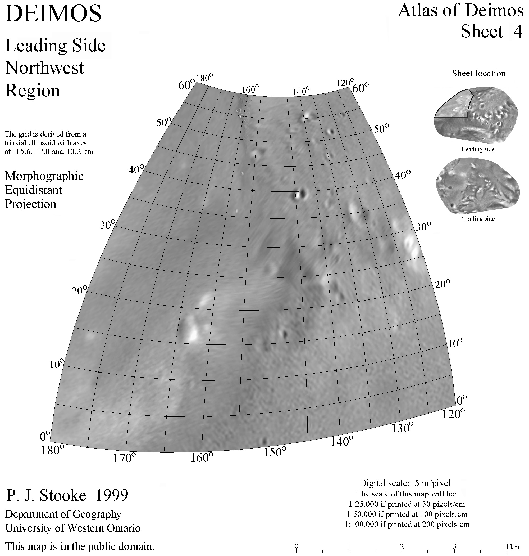
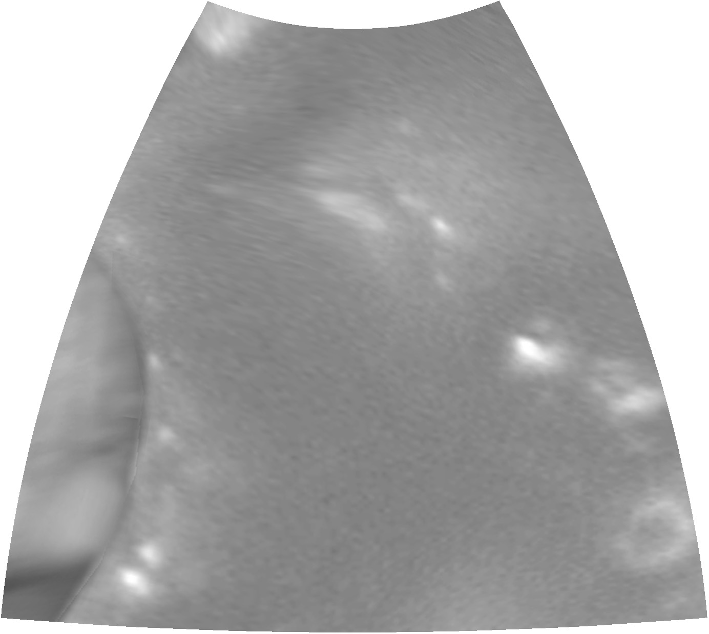
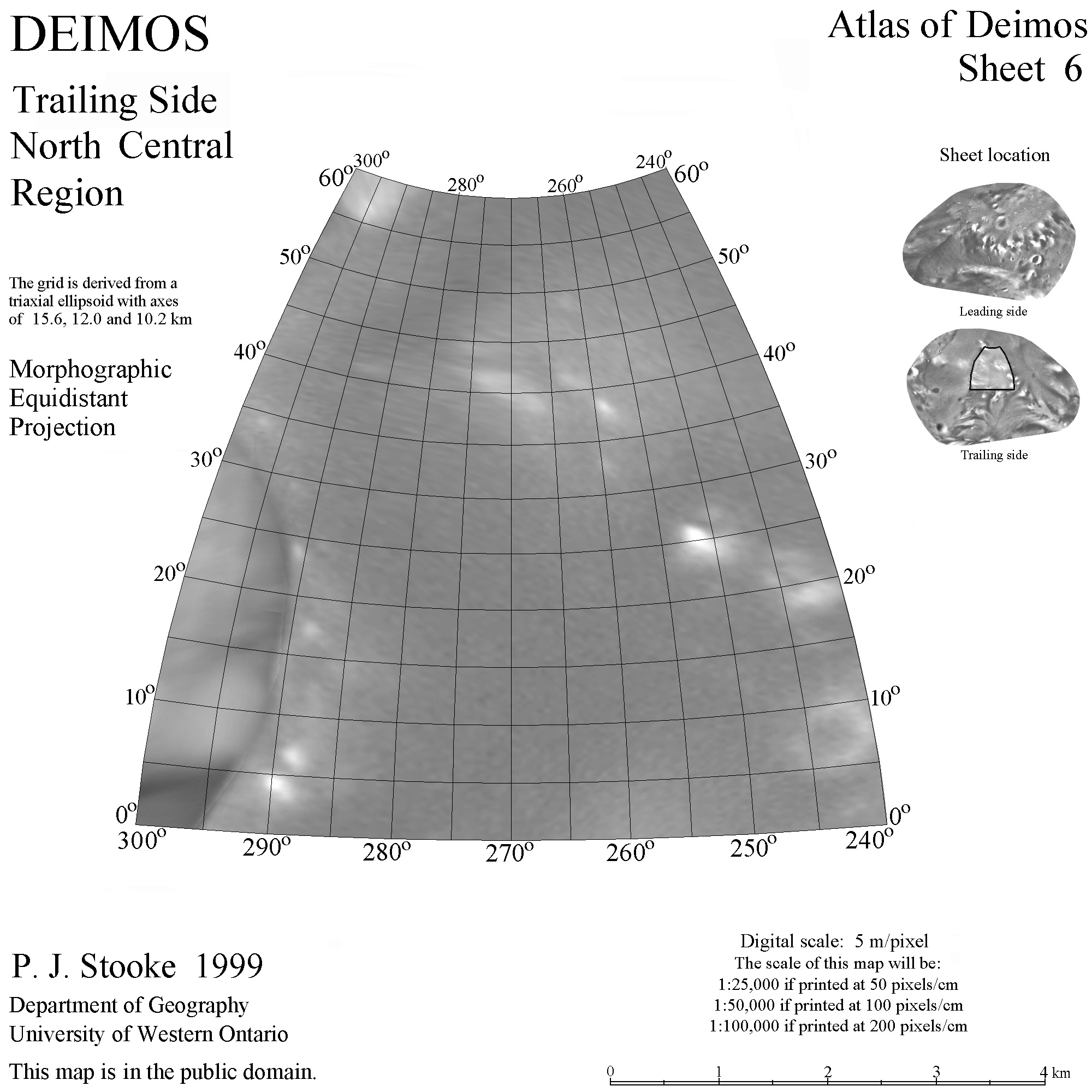
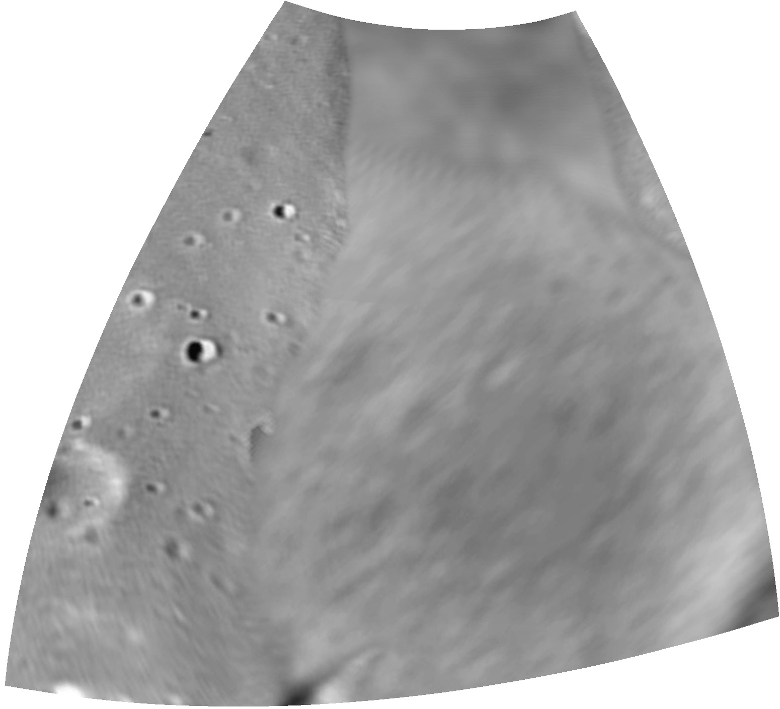
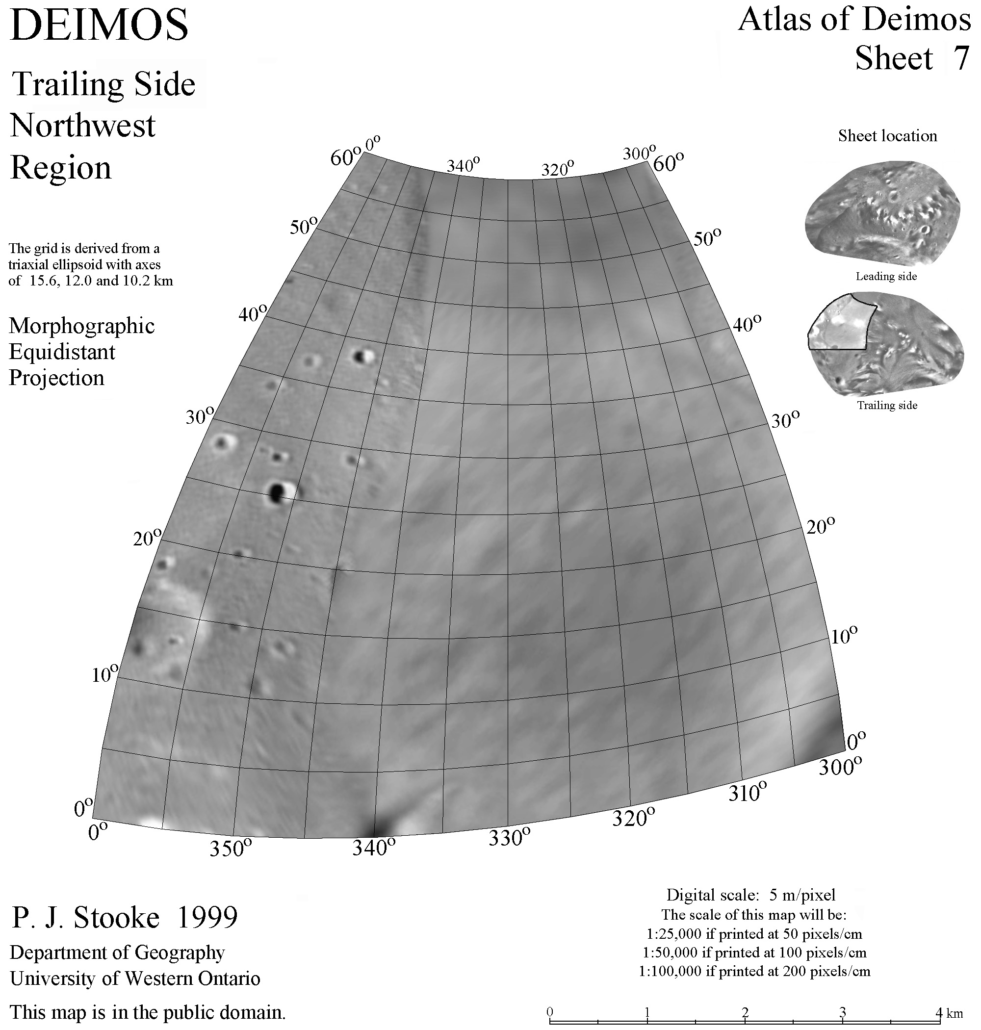
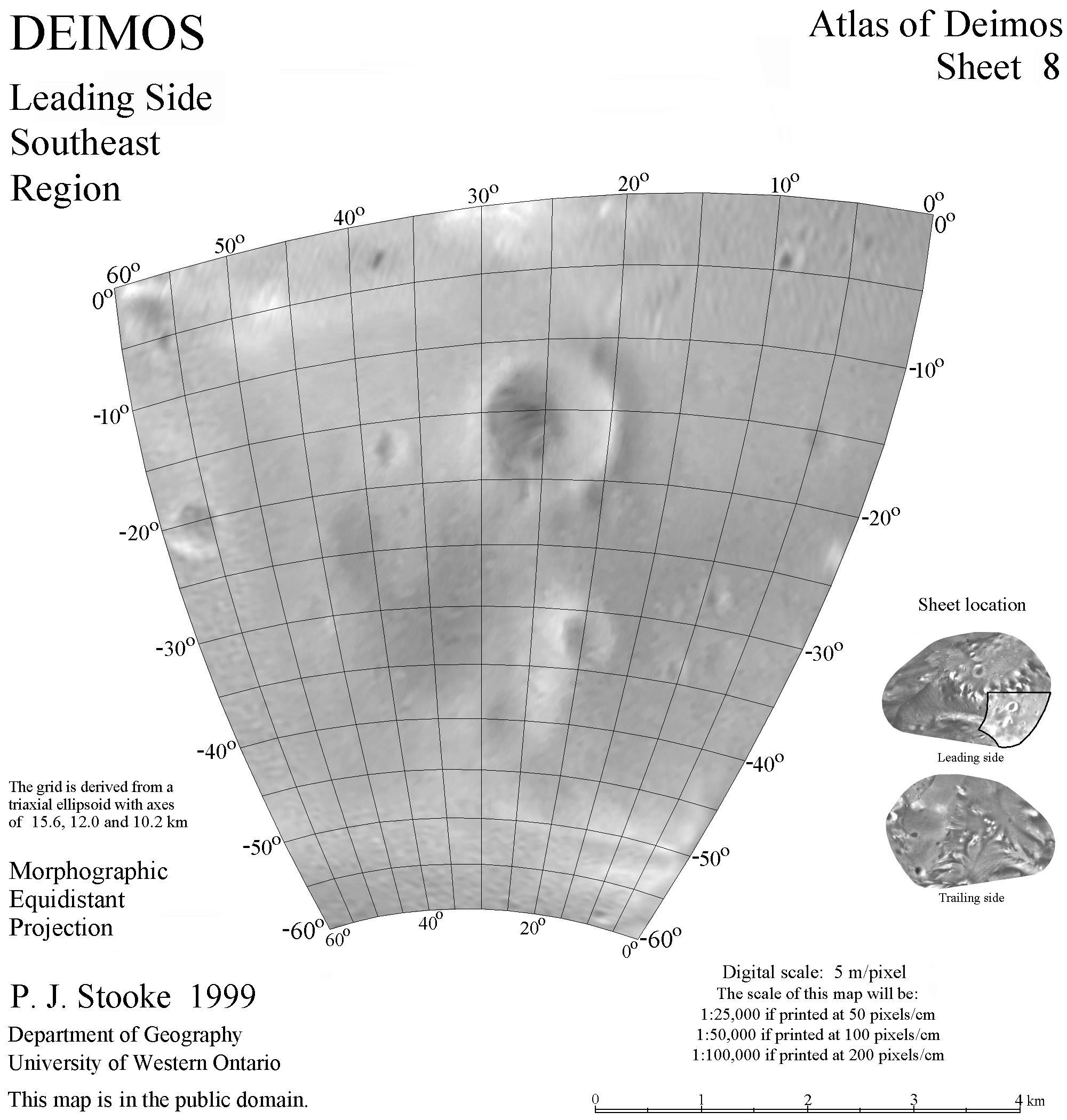
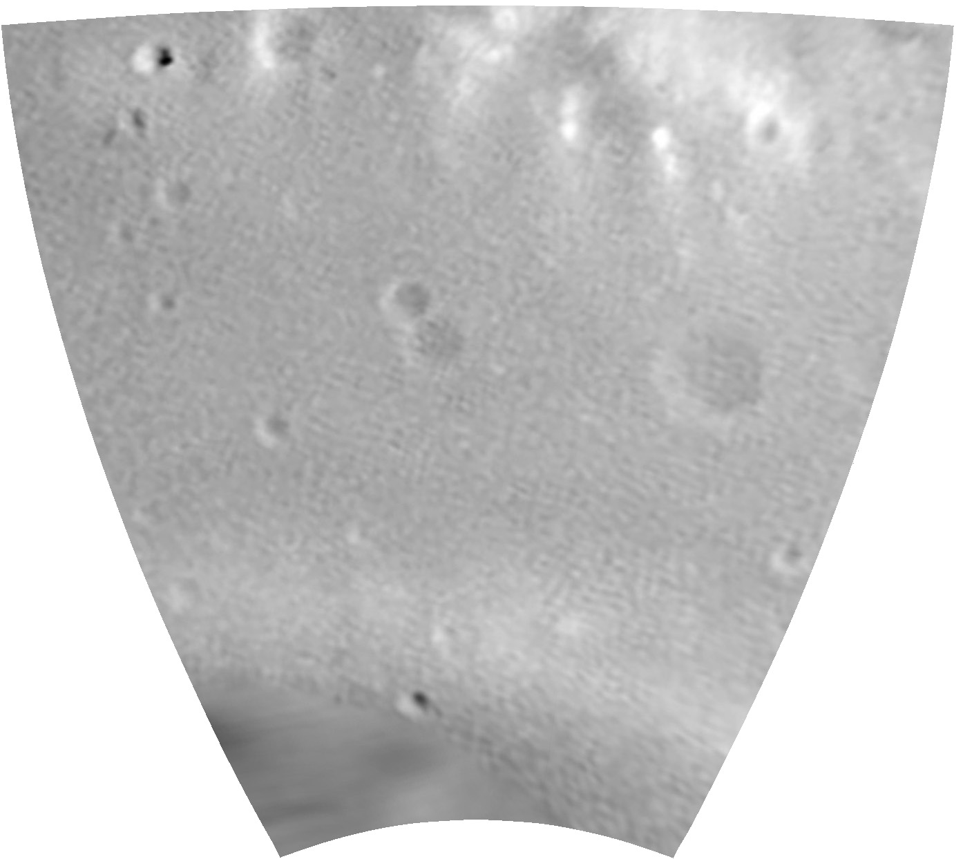
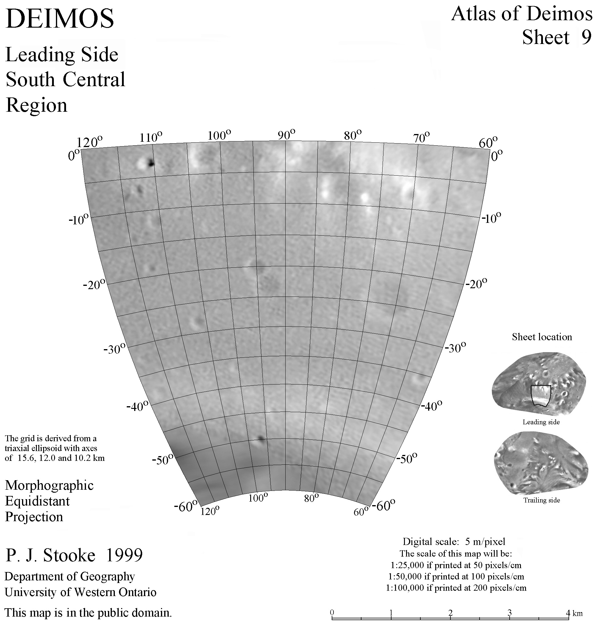
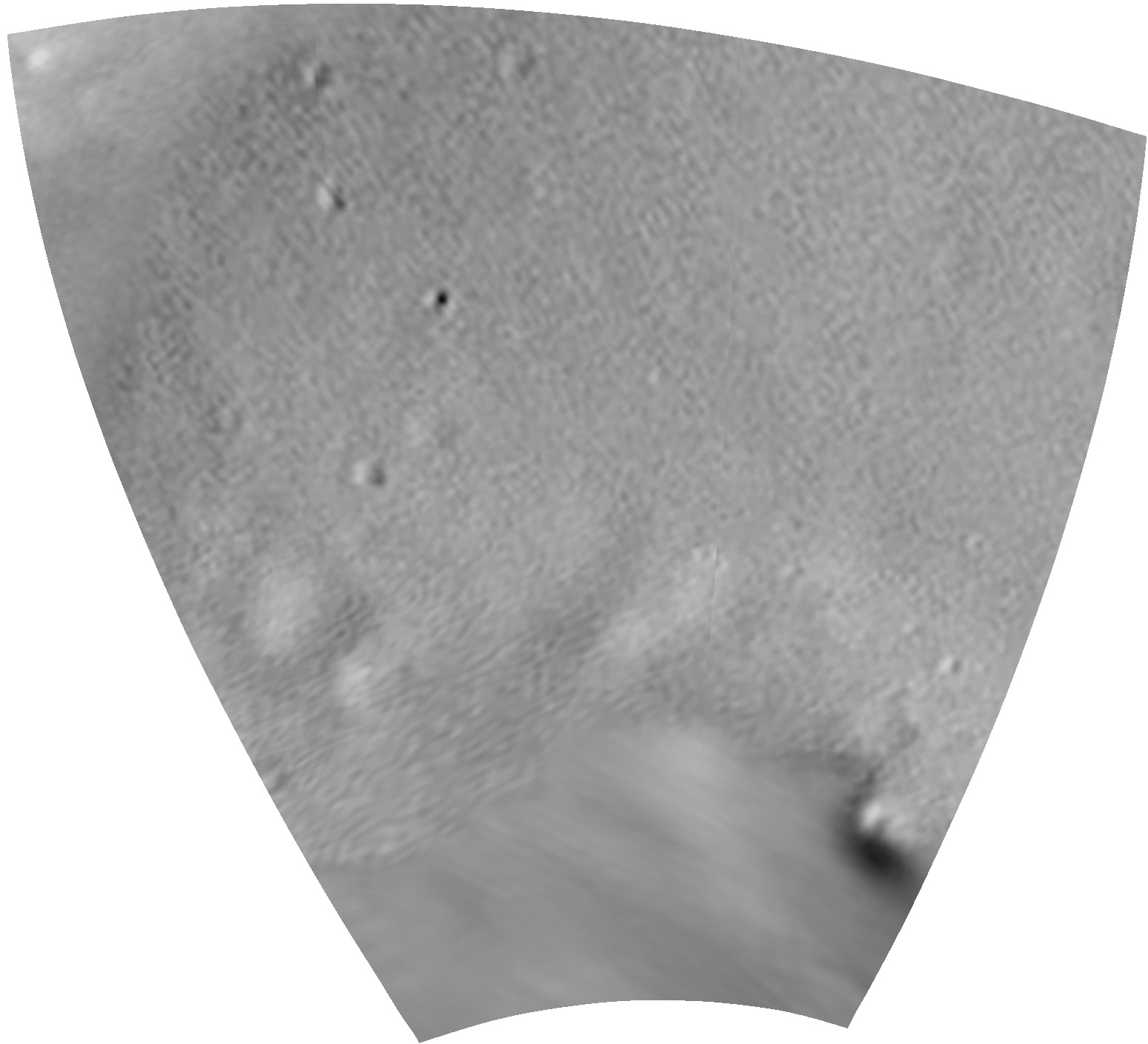
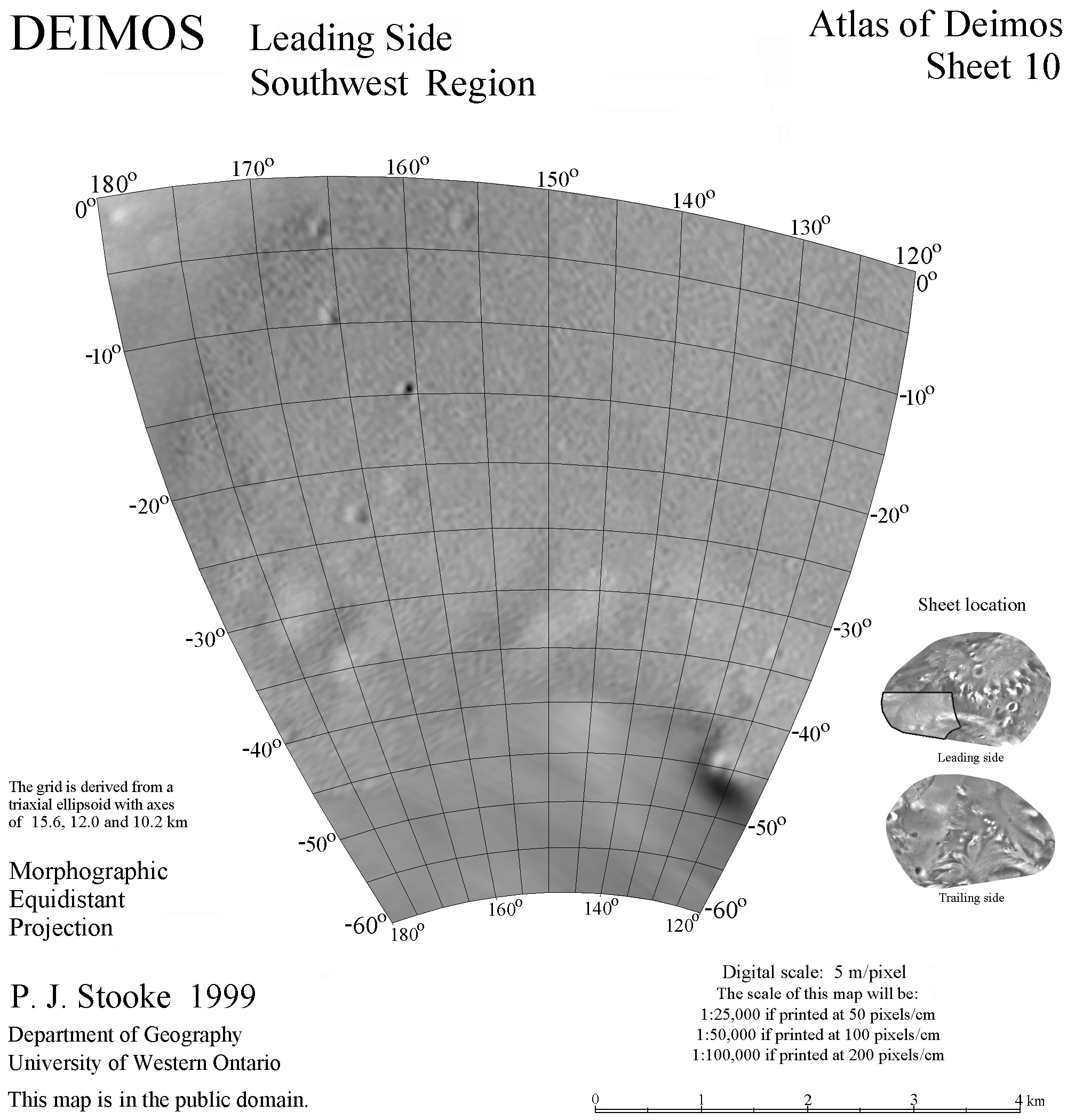
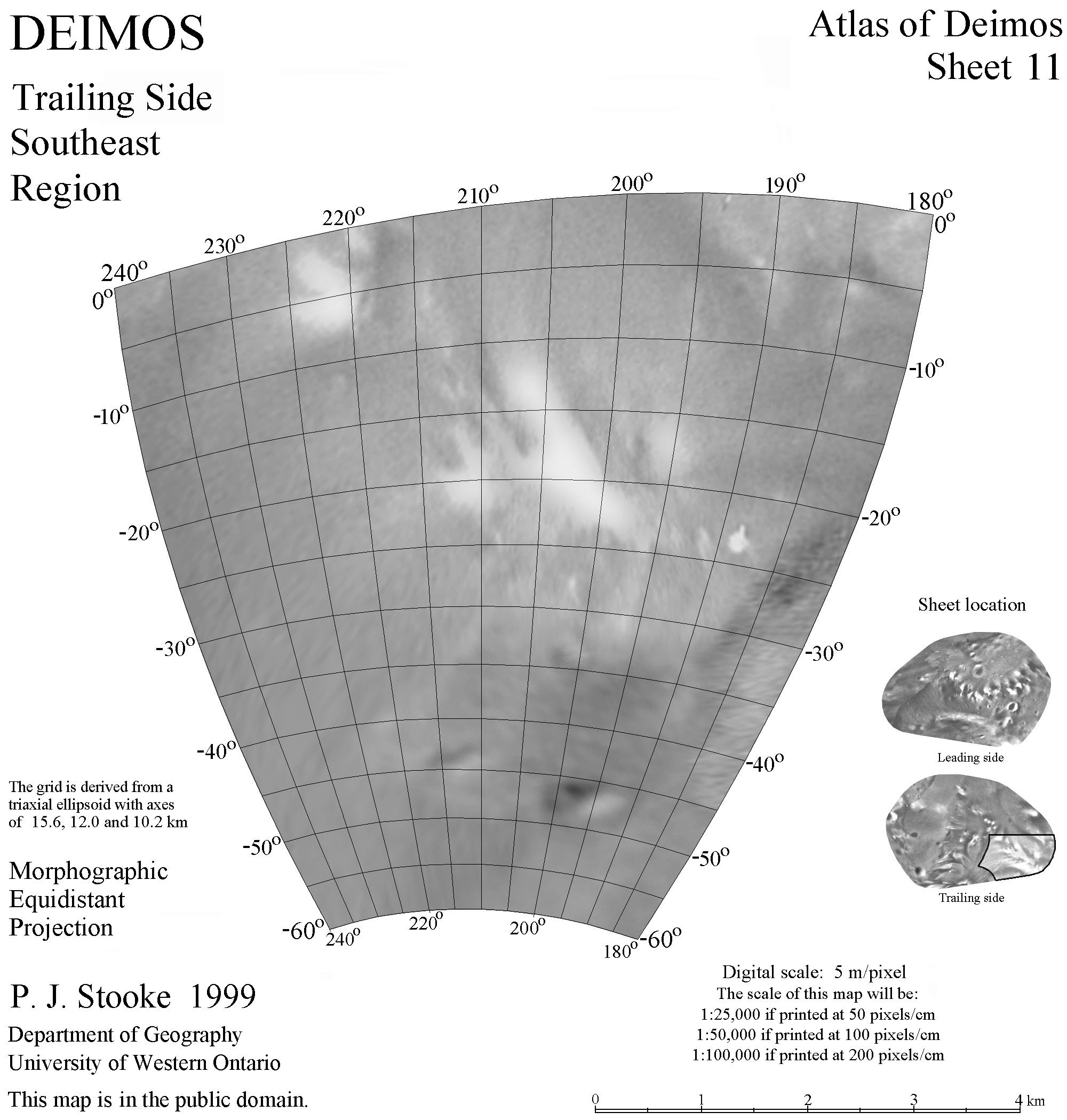
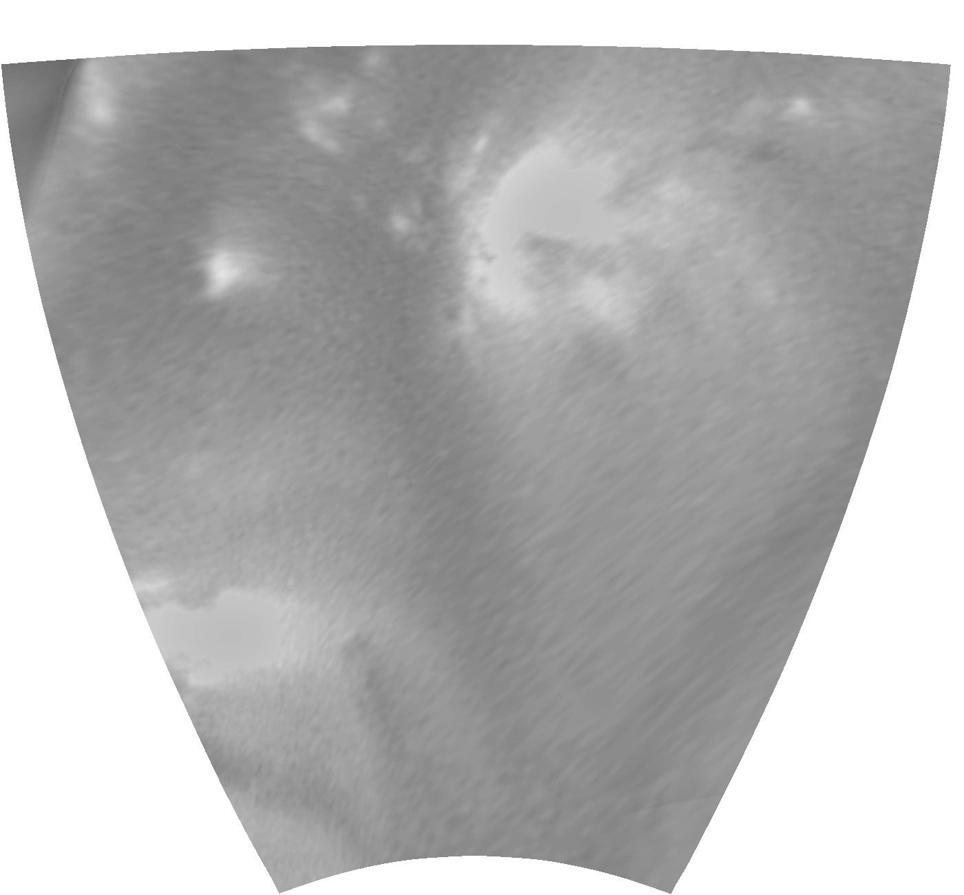
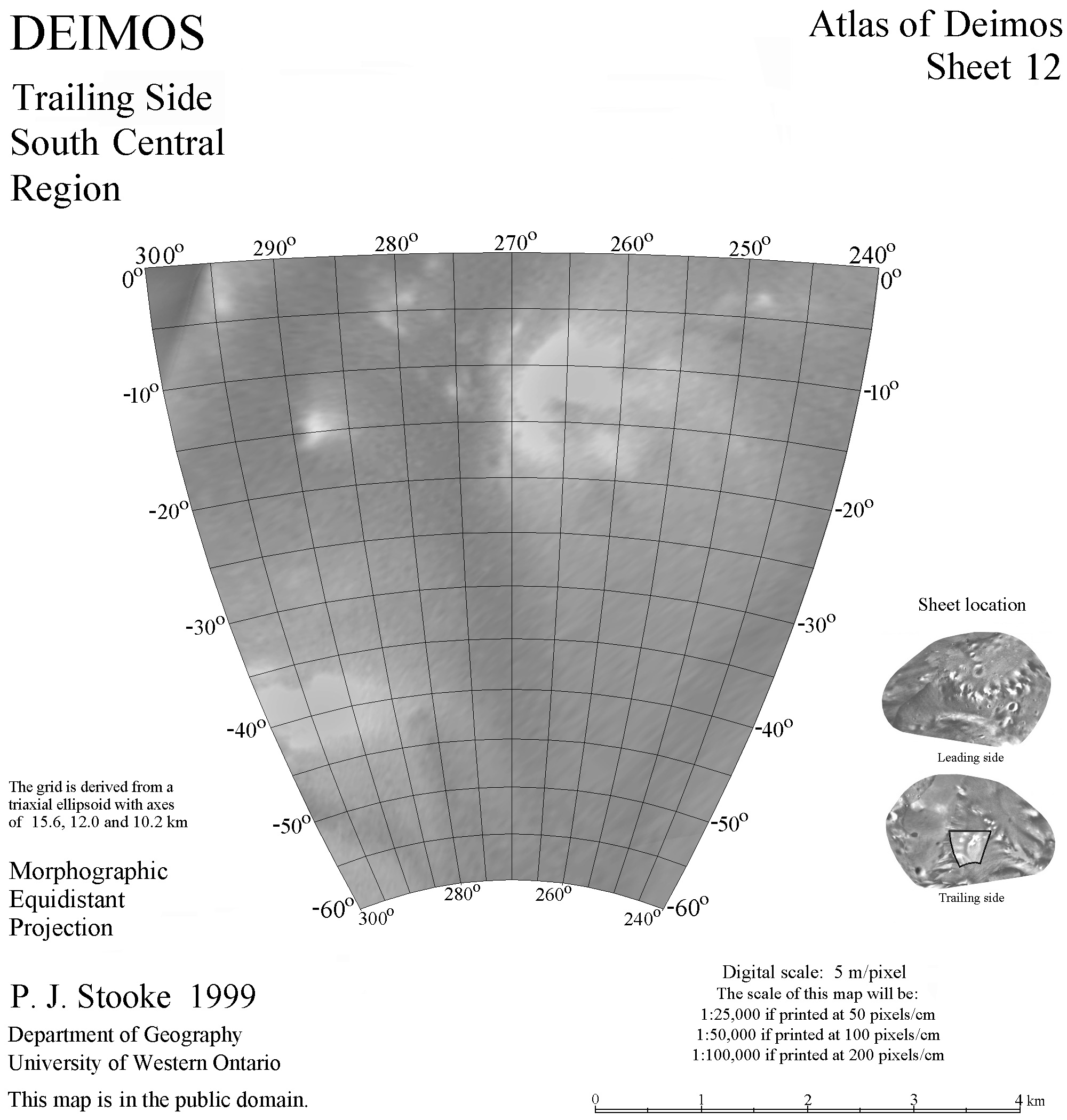
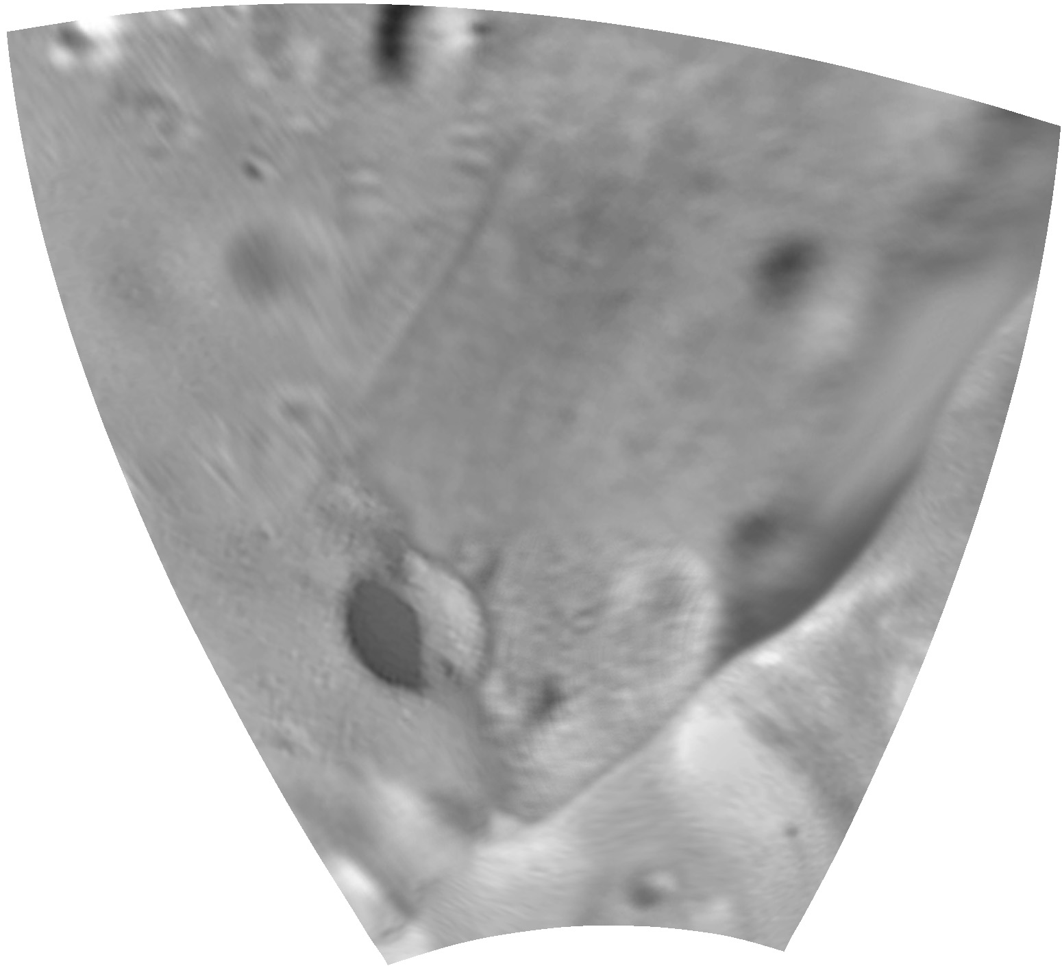
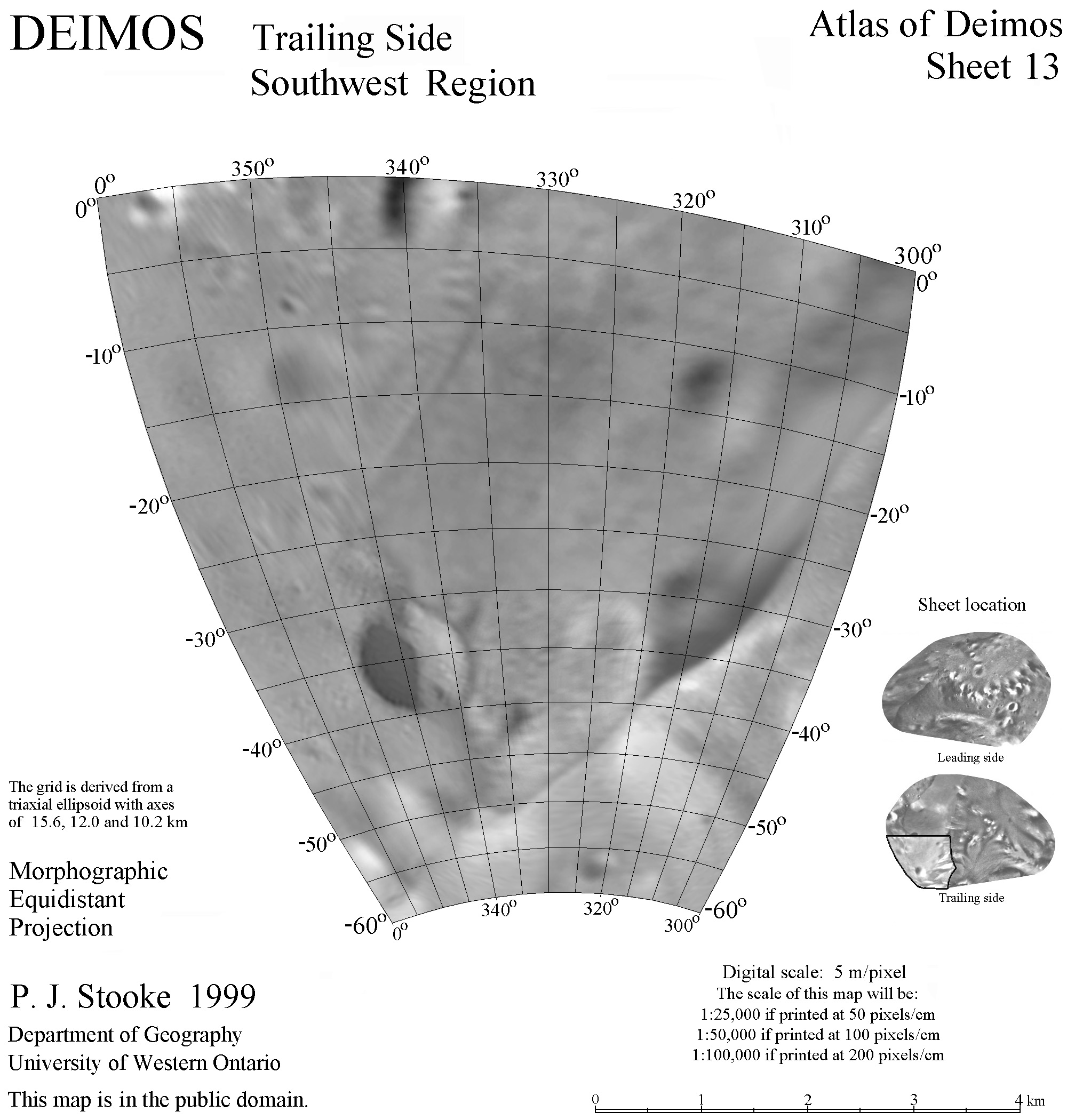
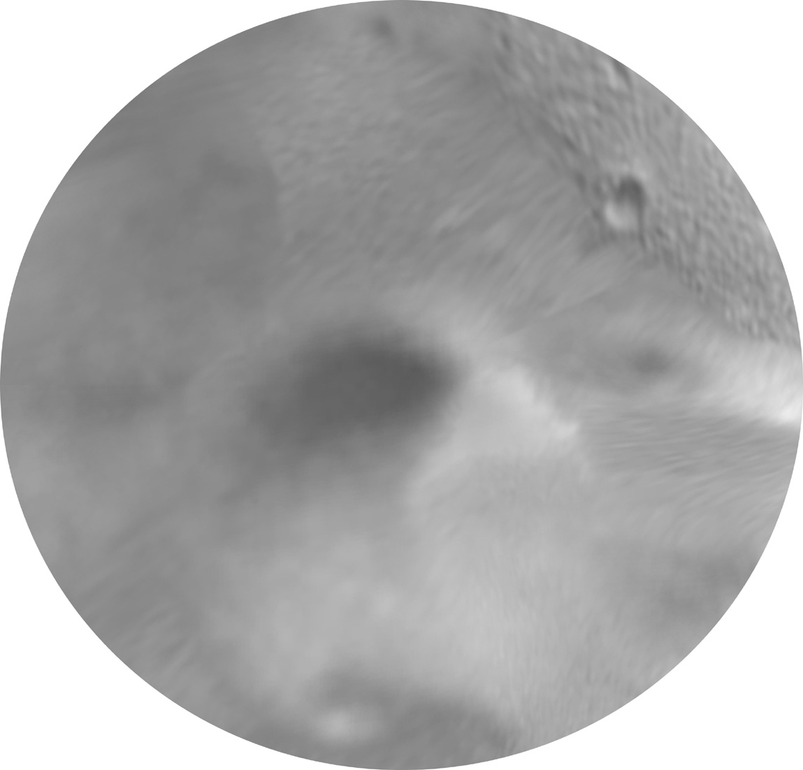
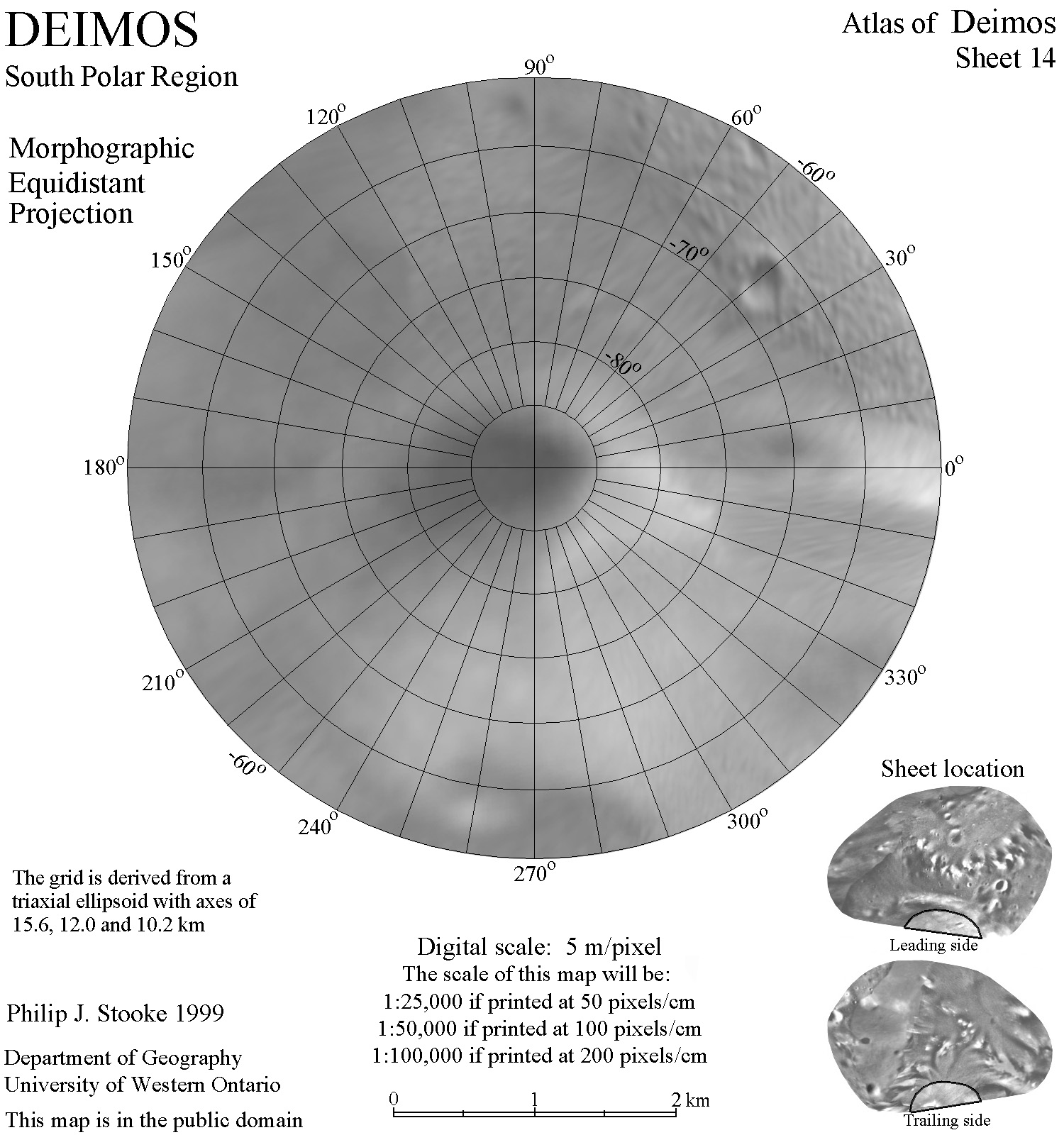
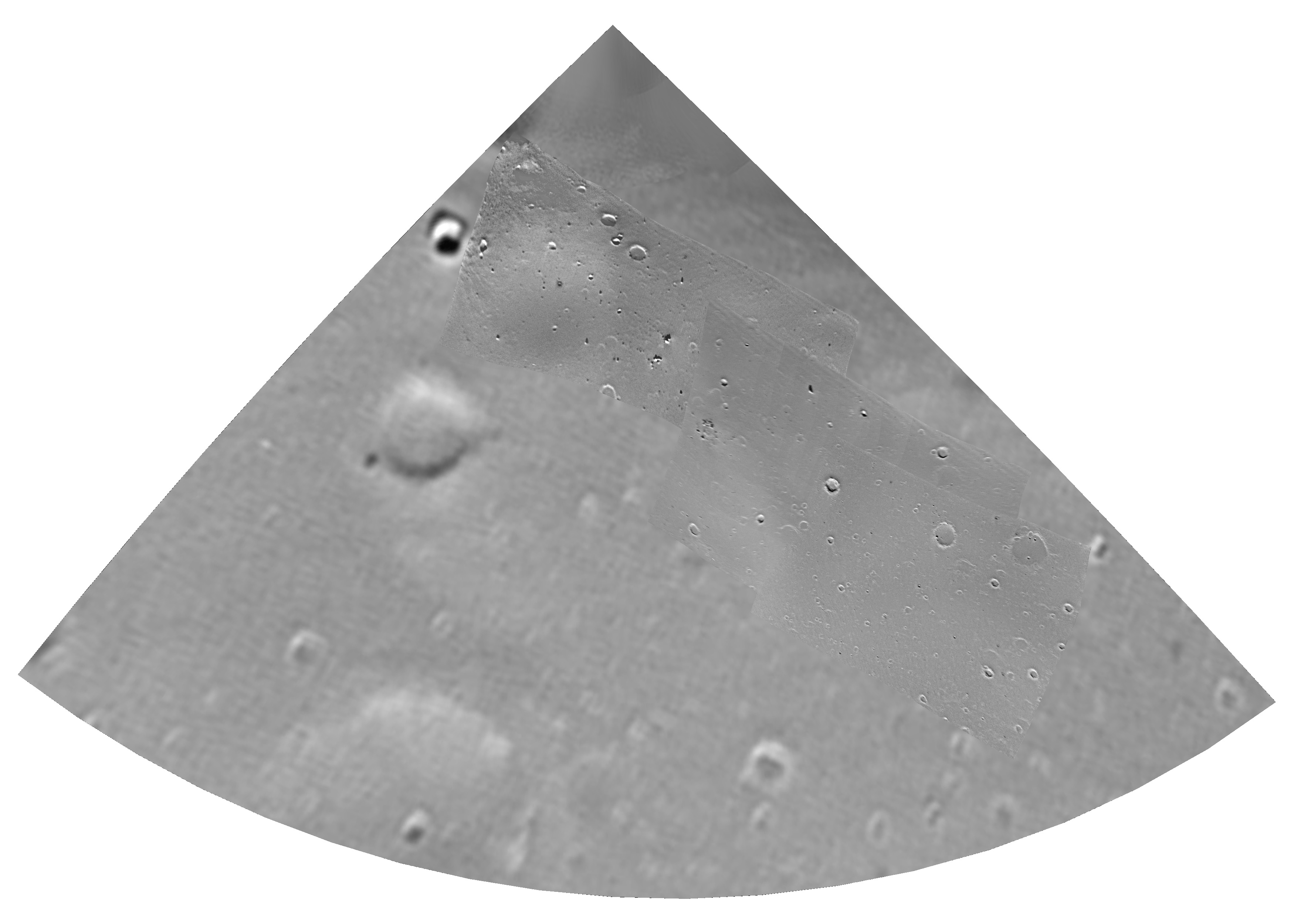
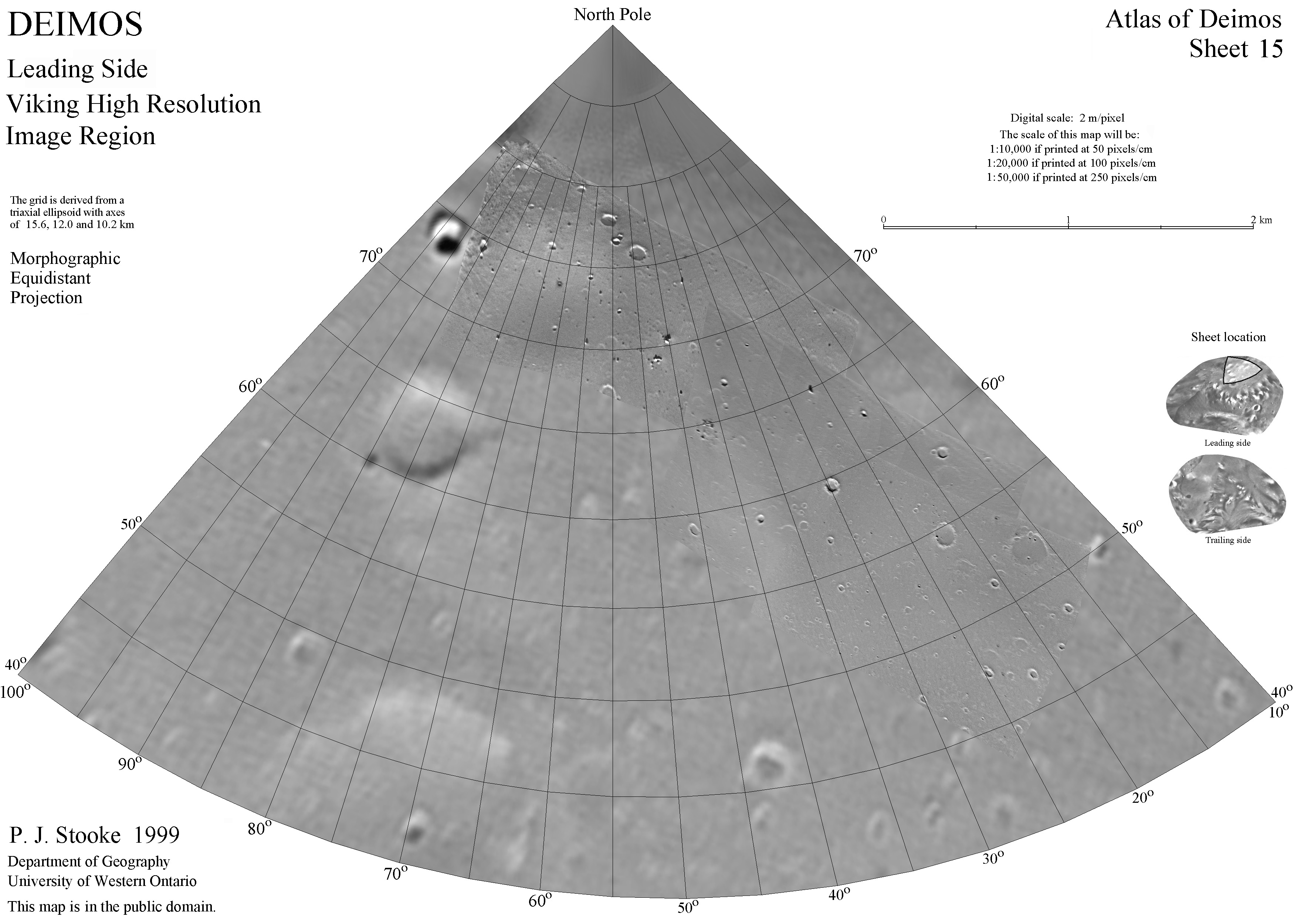
A. Photomosaics of Deimos created from the original Viking and Mariner 9 images by Philip Stooke with the assistance of Chris Jongkind and Megan Arntz. Control is based on a shape model and mosaic by Peter Thomas and colleagues at Cornell University, to whom the author is very grateful for permission to use them. The photomosaic was compiled on a Simple Cylindrical Projection, then reprojected to a map projection designed for use with non-spherical bodies. The map grids are derived from a best-fit triaxial ellipsoid whose dimensions are given on each map.
These maps cover all of Deimos in 14 sheets, each 60 degrees by 60 degrees,
sheet limits shown on labelled and gridded versions. The fifteenth sheet
covers a special high-resolution area.
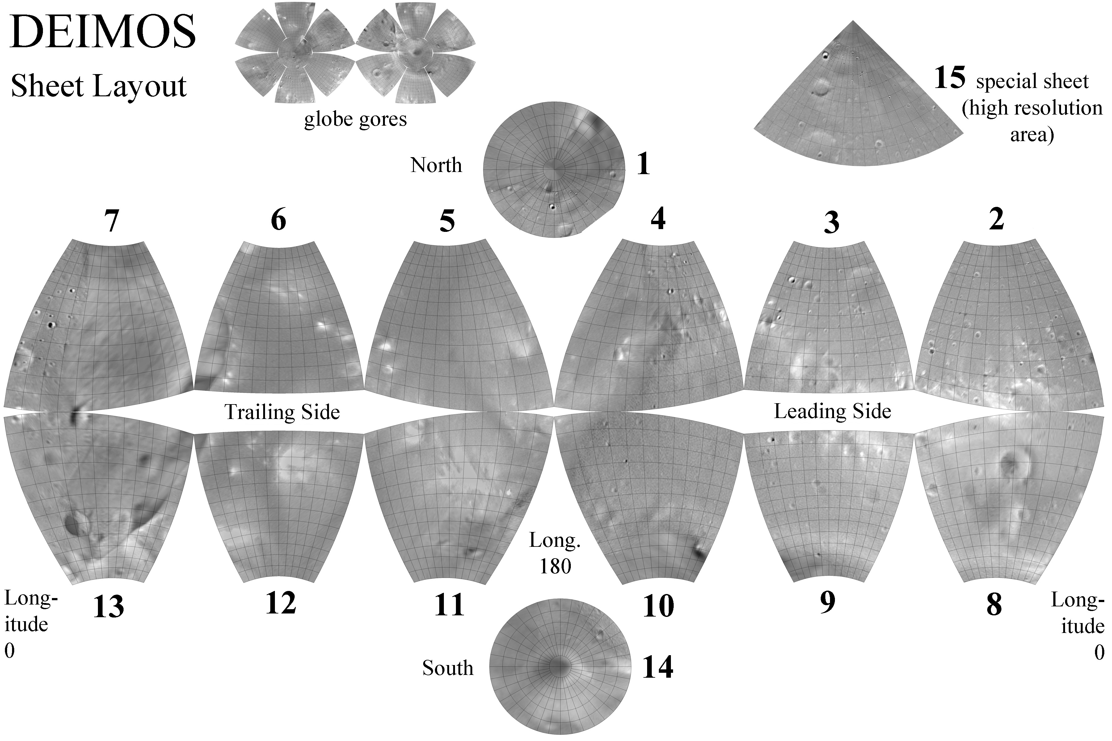
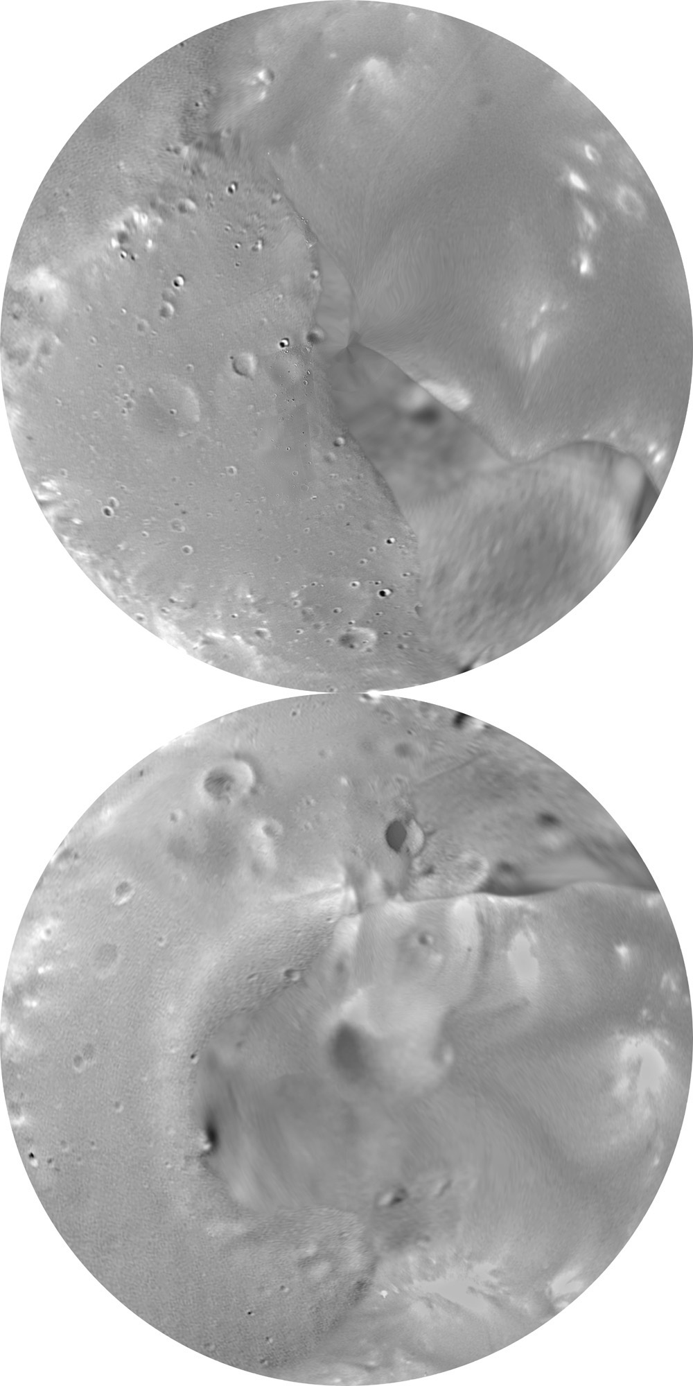
B. Globe gores: Composites of the gridded sheets above arranged around the polar sheets in separate northern and southern hemispheres. These may be cut out and assembled to make a globe, not perfectly shaped but interesting.
Sheet showing the layout of the above-listed set of Deimos maps.
C. Global mosaics in various projections, created by Philip Stooke with the assistance of Chris Jongkind and Megan Arntz. The Mariner 9 mosaic was produced with the assistance of John Pfau. Control is based on a shape model and mosaic by Peter Thomas and colleagues at Cornell University.
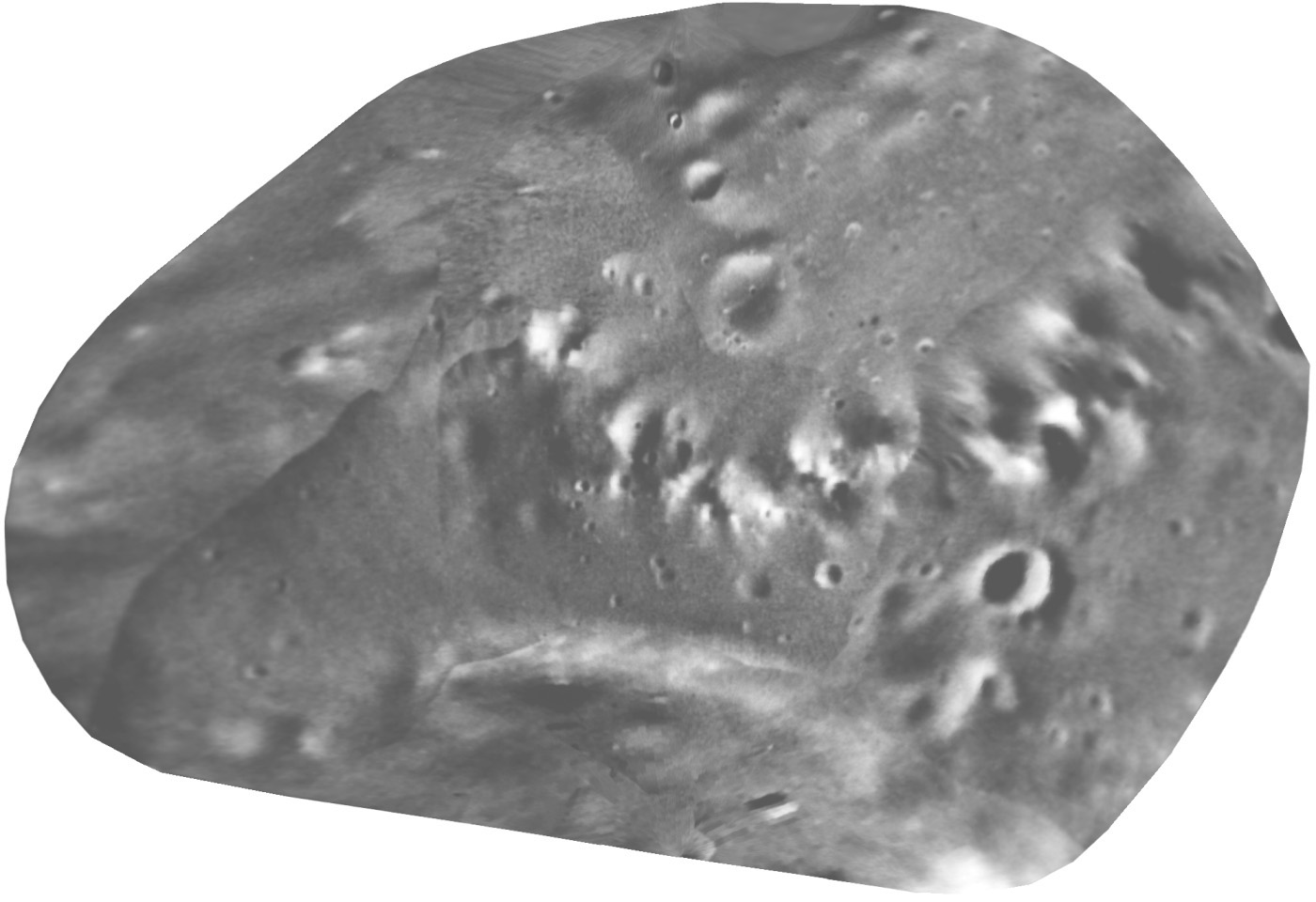
D. Enlarged and modified version of the Simple Cylindrical Projection Mosaic listed above, with the addition of details from Mars Reconnaissance Orbiter HiRISE images ESP_012065_9000 and ESP_012068_9000 and some geometric improvements near 60 East longitude at the equator.
Simple Cylindrical Projection , north at the top, 0 longitude at the center, 7200 by 3600 pixels. (20 pixels/degree)
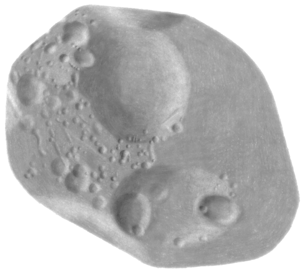
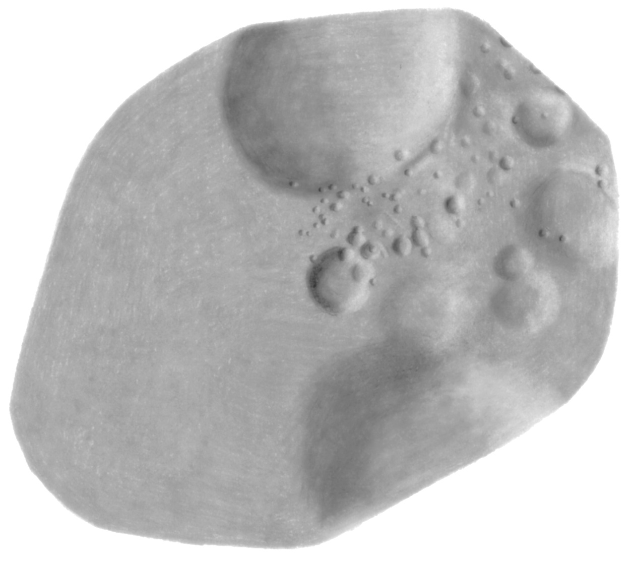
These shaded relief maps were drawn by P. Stooke from Voyager images of Amalthea, positional control by P. Stooke. The maps are derived from an original drawing in a different projection which was included on the Galileo mission web site at JPL. Here, the original drawing has been converted to Simple Cylindrical projection at 10 pixels/degree, and then reprojected to other projections.
Note on the Prismographic Projection (P. Stooke, unpublished, 1999): The spacing between meridians is equal to their spacing (at the equator) on a triaxial ellipsoid used as a shape model (131 x 73 x 67 km semiaxes). The spacing between parallels is equal to their spacing along each meridian on the triaxial ellipsoid. Different variants, approximating equivalence, equidistance, and conformality, would be possible if appropriate scale factors are introduced in the y coordinate equations. In the case illustrated here the y coordinates are divided by the cosine of the latitude, which increases spacing towards the poles to give a compromise between equidistance and conformality. The name "prismographic" indicates that the surface is projected onto a prism with the same cross section as the body's equator. Cylindrical projections are a subset of prismographic projections. Extends from 70 degrees north to 70 degrees south.
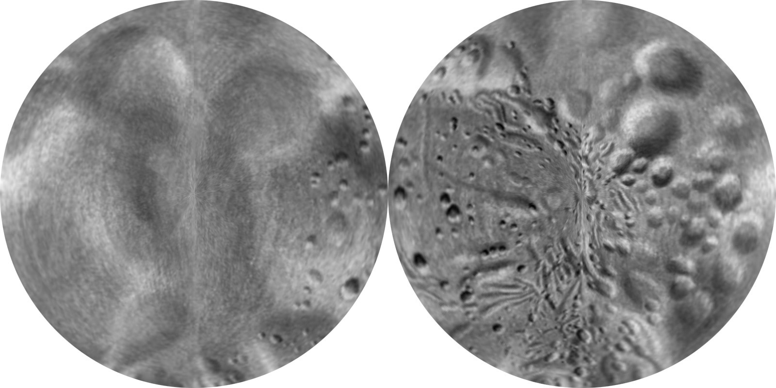
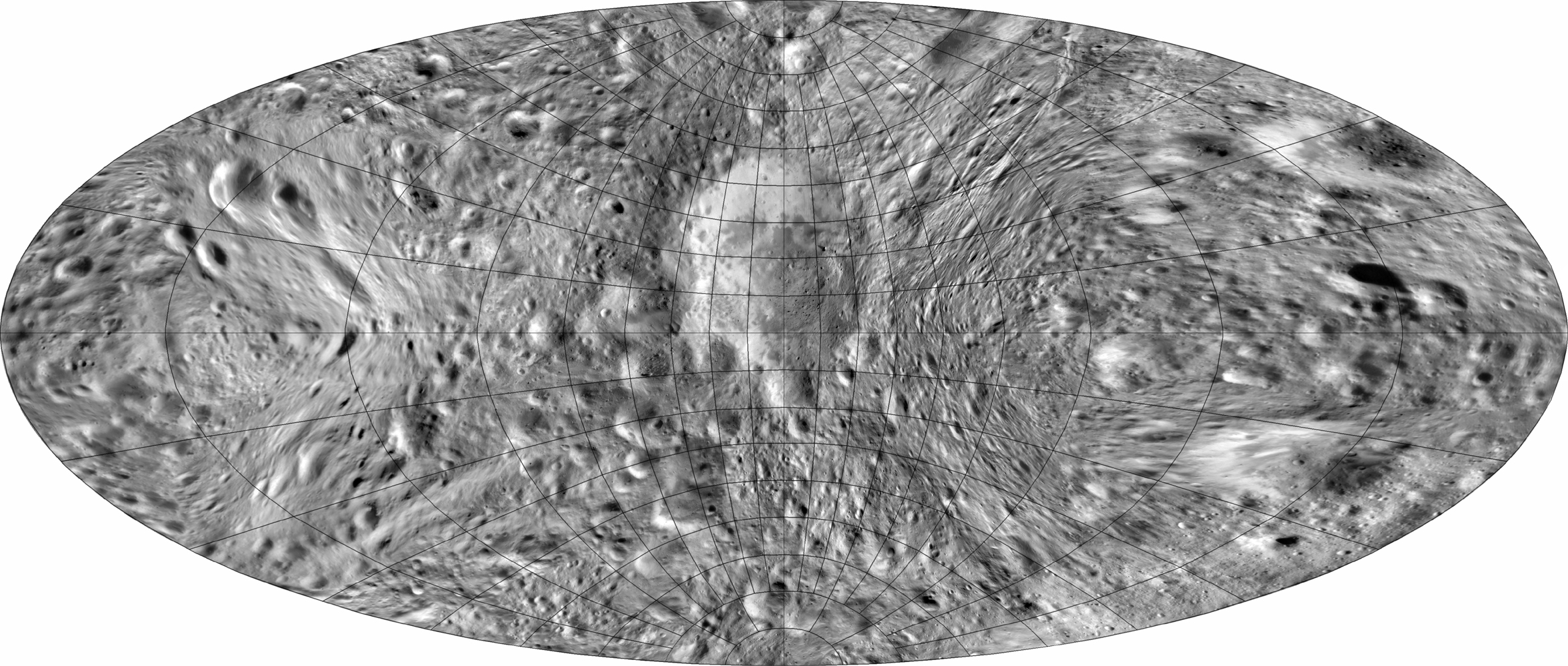
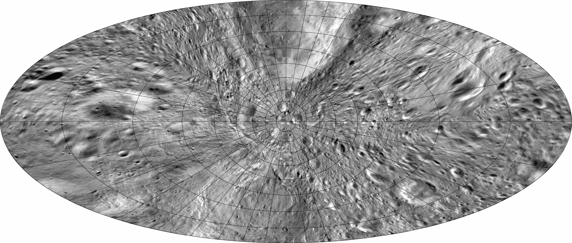
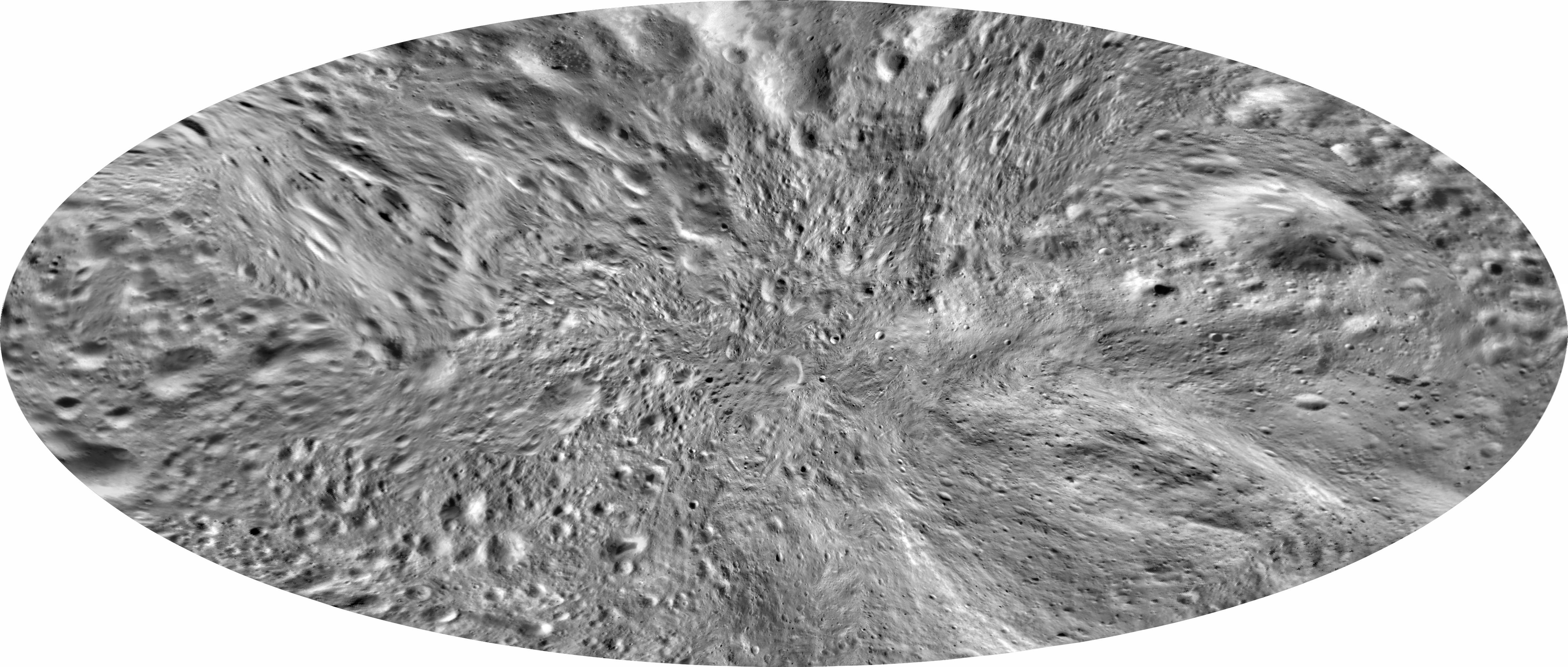
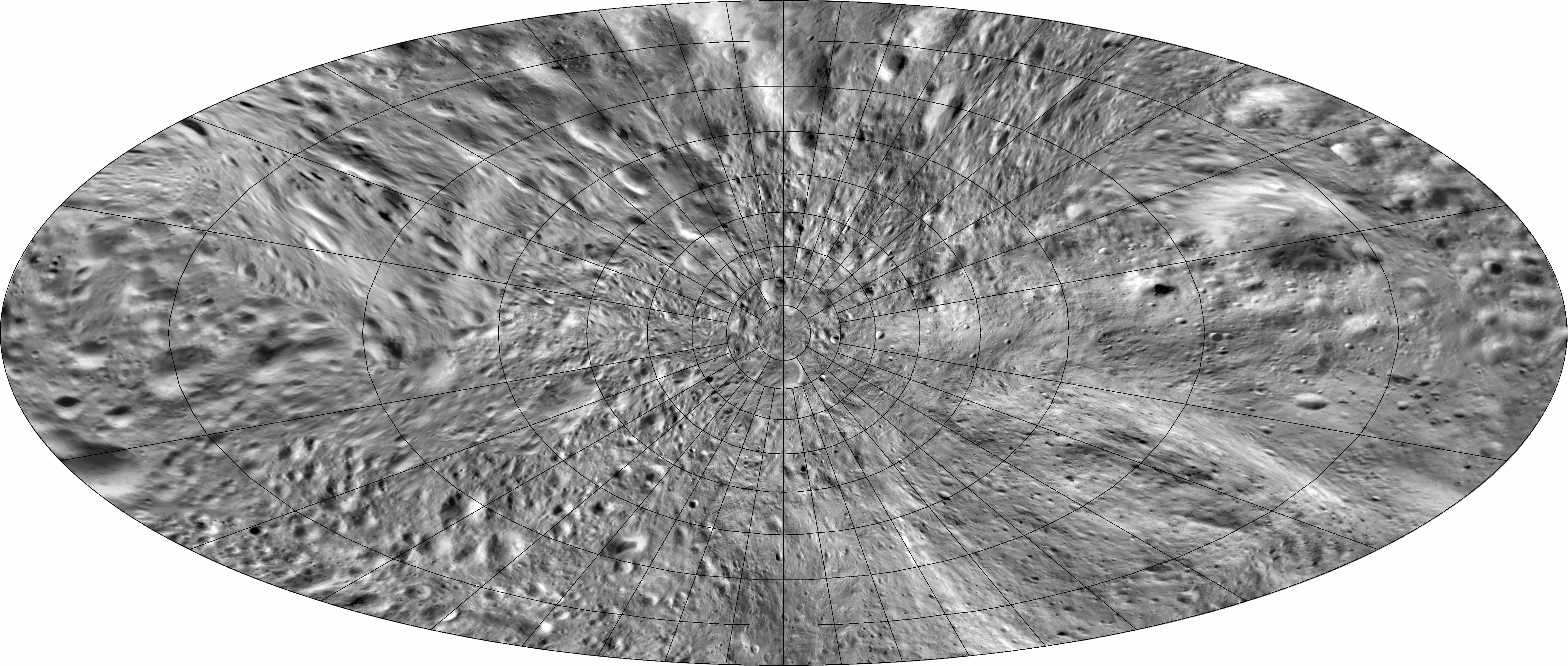
Shaded relief maps of Hyperion, based on Voyager 2 images, using control by P. Thomas.
Note: Morphographic Conformal projection is shaded relief drawing projected onto the 3D convex hull of the shape, then reprojected to morphographic conformal (effectively stereographic) projection, in two hemispheres centered on the equator and at longitudes 90 and 270.
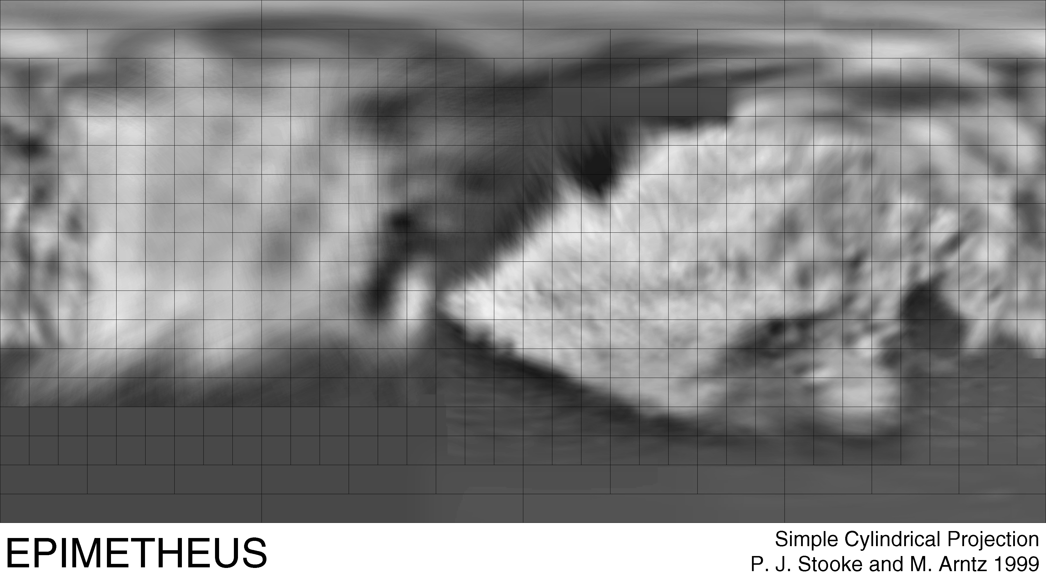
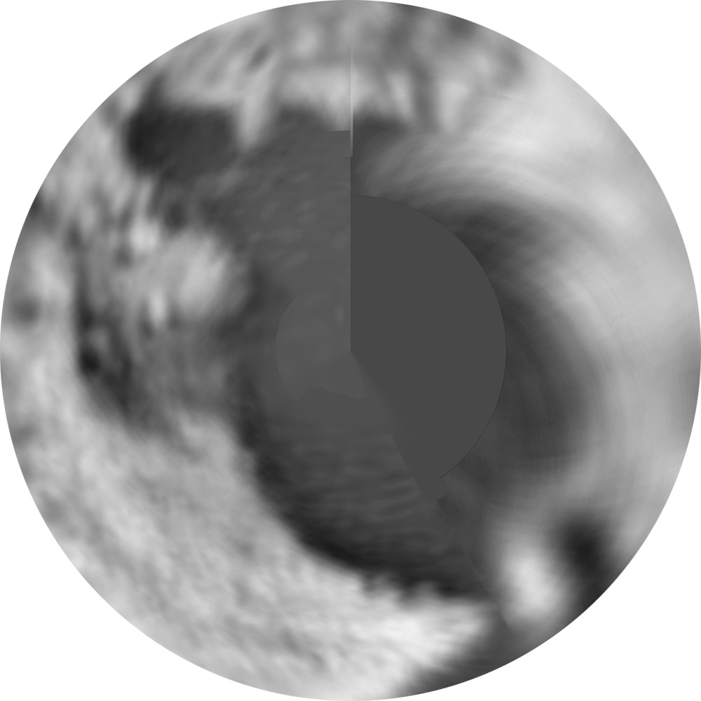
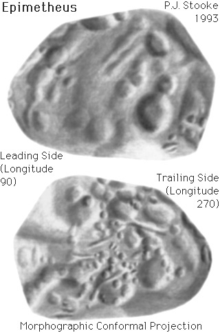
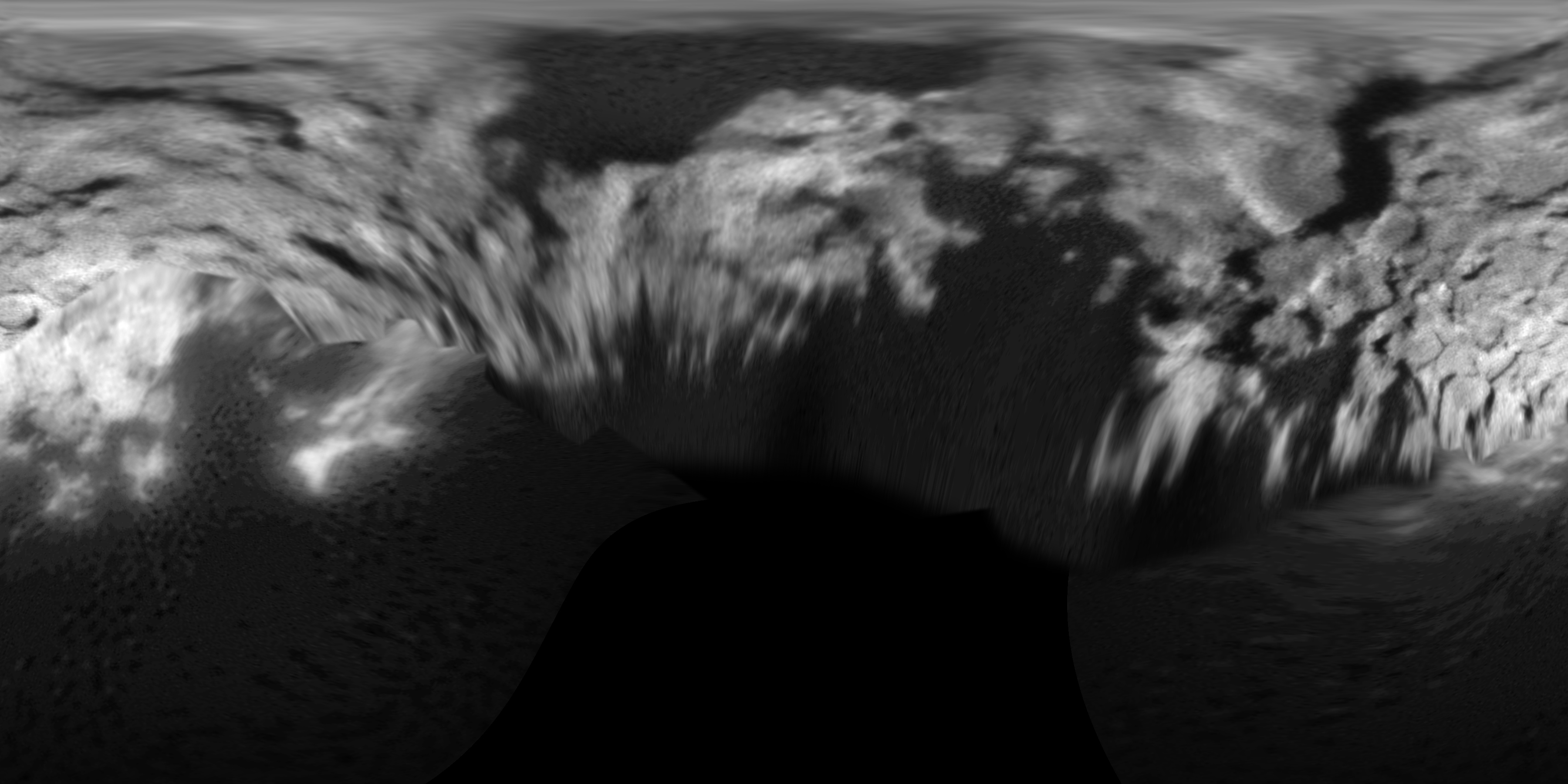
Maps and mosaics of Epimetheus based on Voyager 1 and 2 data. Control in the mosaics is by P. Thomas, but in the shaded relief map it is from an earlier, less reliable shape by P. Stooke.
Note: Morphographic Conformal projection of a shaded relief drawing projected onto the 3D convex hull of the shape, then reprojected to morphographic conformal (effectively stereographic) projection, in two hemispheres centered on the equator and at longitudes 90 and 270.
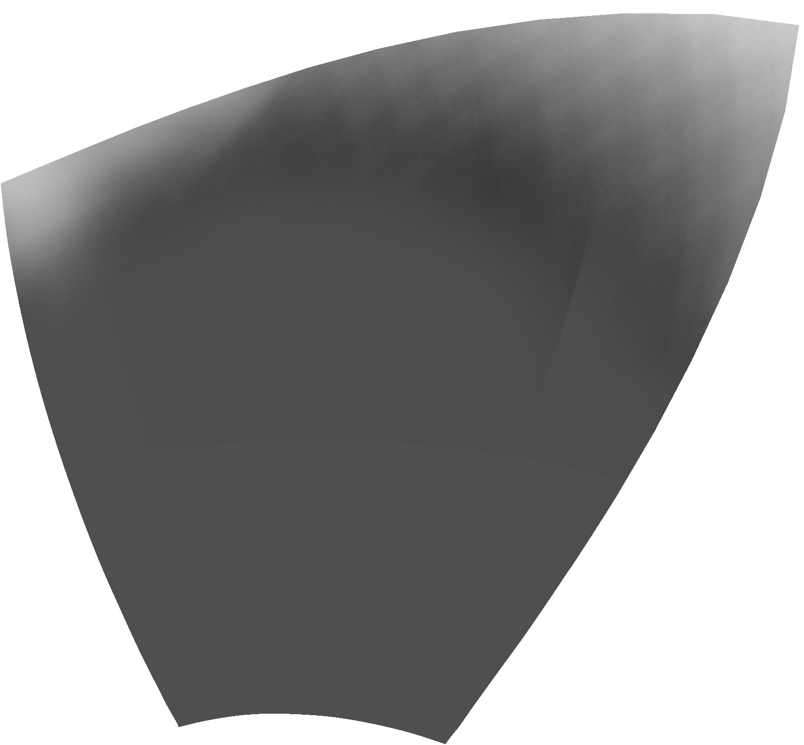
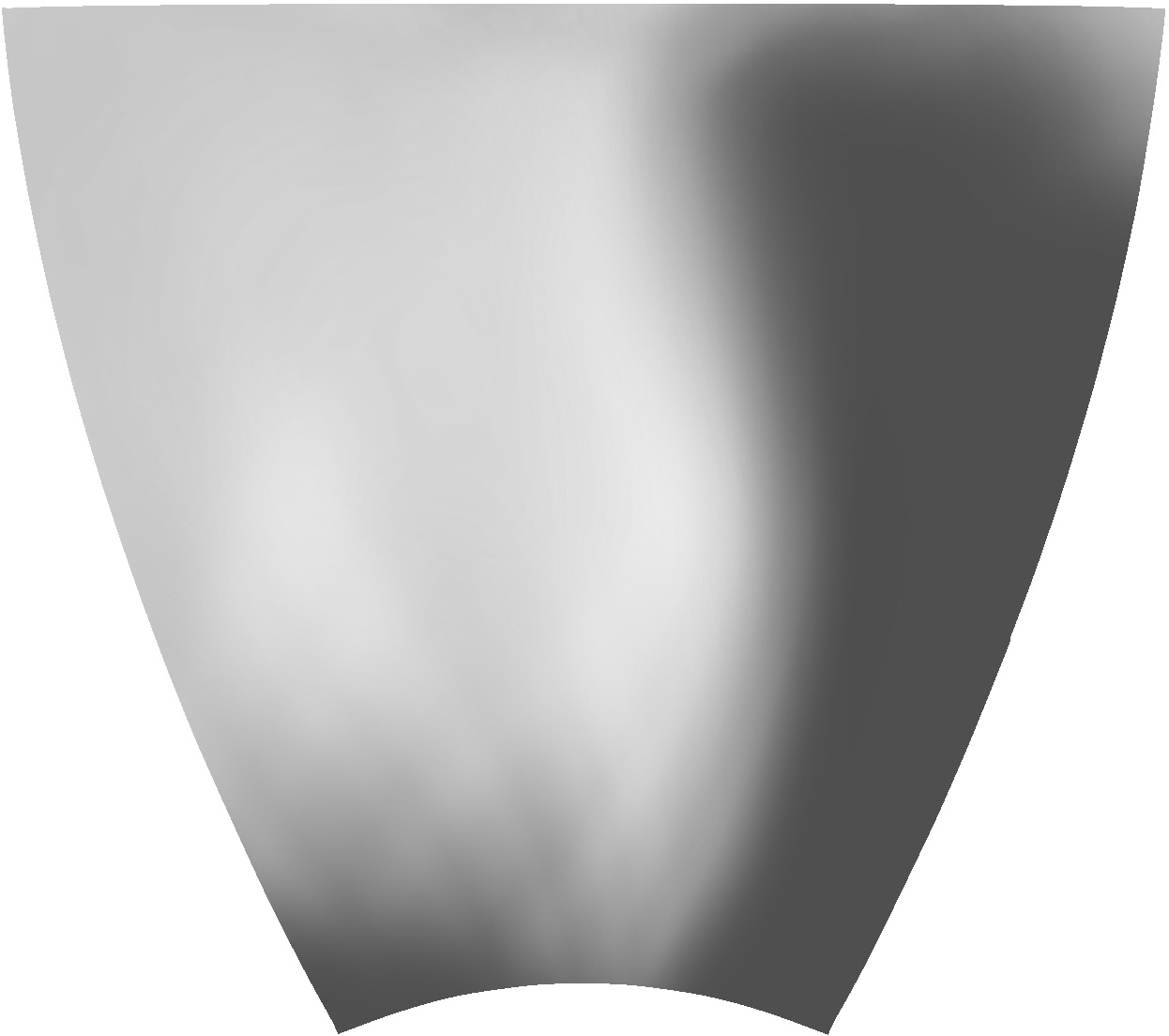
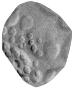
These maps are based on the results described by Duxbury et al. (2004). That paper includes Stardust images of the Wild-2 nucleus with superimposed ellipsoidal grids, and a small polar stereographic and cylindrical projection map.
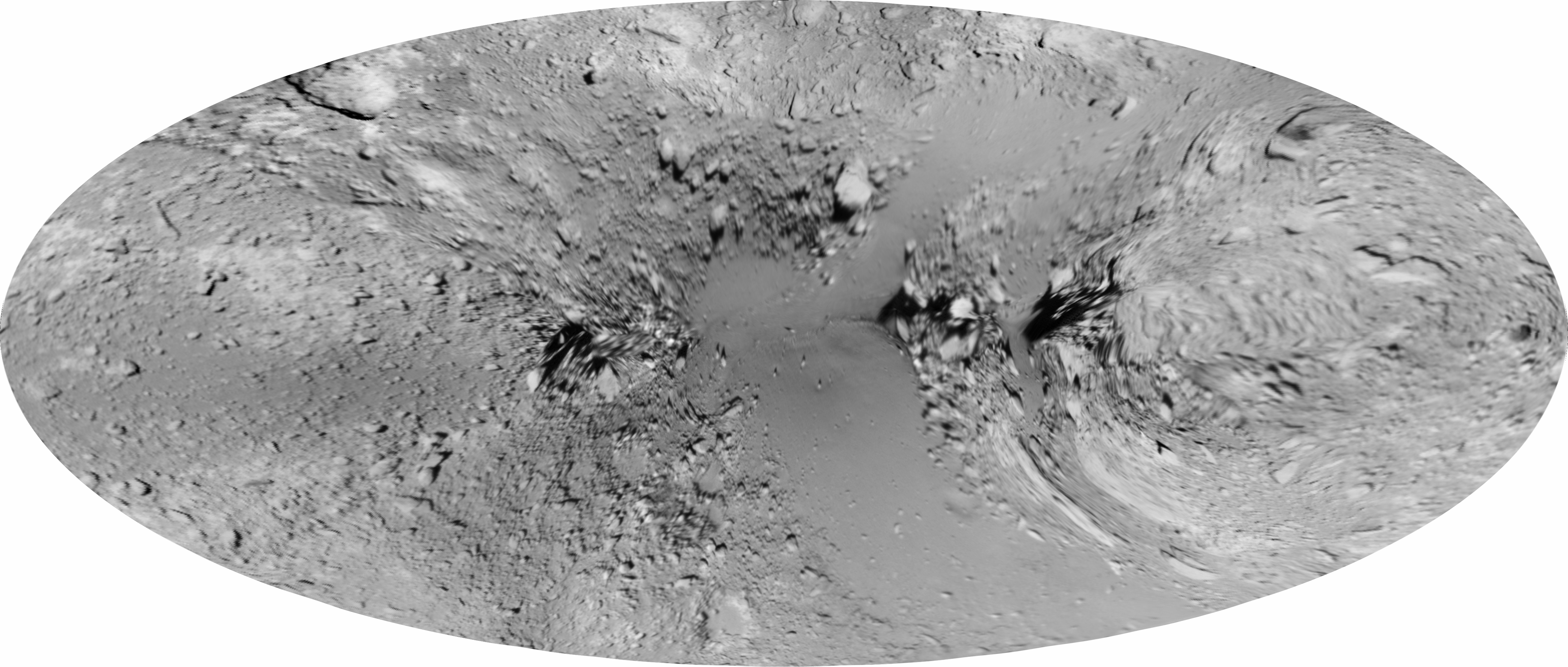
The original Stardust images were reprojected using the geometry of the ellipsoidal grids and combined to make a photomosaic of the northern hemisphere. The reprojection does not make use of a high fidelity topographic model, so accuracy is limited and difficult to quantify. Positional errors of up to 10 degrees may occur.
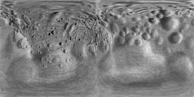
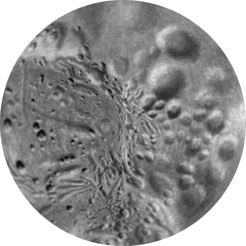
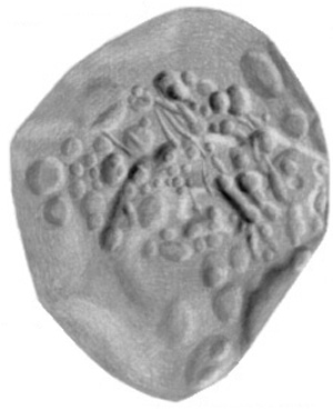
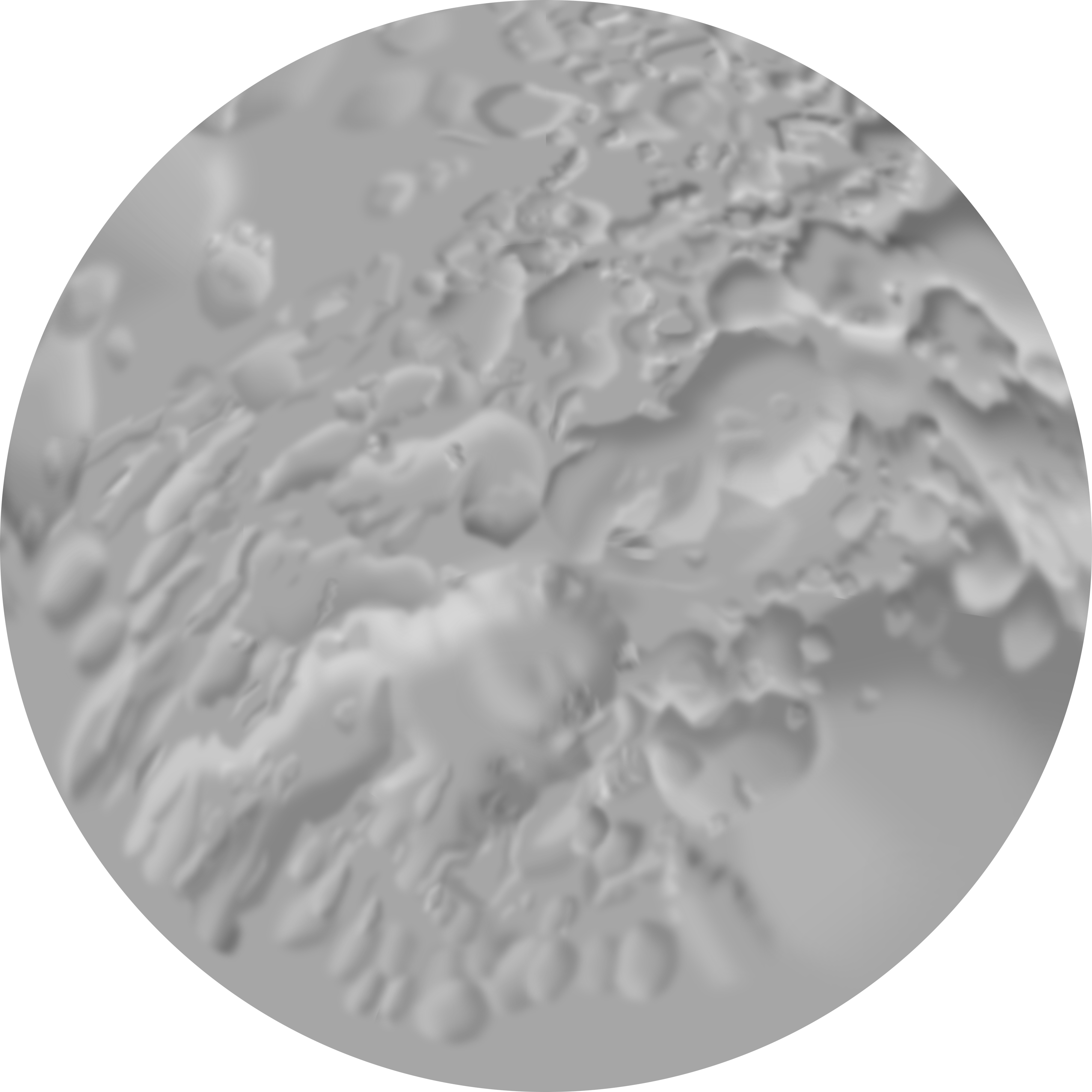
The second map is a shaded relief interpretation of the photomosaic. Such interpretations are always subject to some uncertainty, especially where illumination runs along a slope rather than across it (i.e. along the strike of a slope rather than across the dip of the slope, in stratigraphic terms). It may be useful for visualization of jet sources.
These maps are offered as aids to visualization where a global map in conventional coordinates is required. They may be useful since there are no other readily available maps.
Photomosaic:
Simple Cylindrical Projection, north at the top, 0 longitude at the left and right edges, 180 degrees at the center, 3600 by 1800 pixels. (10 pixels/degree)
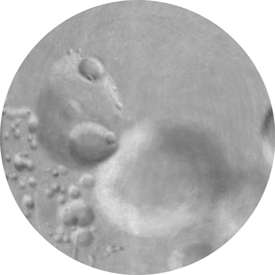
Polar Equidistant Projection (latitudes equally spaced), 0 longitude at the top, north pole at center, equator at the outer edge.
Shaded relief:
Simple Cylindrical Projection, north at the top, 0 longitude at the left and right edges, 180 degrees at the center, 7200 by 3600 pixels. (20 pixels/degree)
Simple Cylindrical Projection - Gridded and labeled version of the above relief map, longitudes increase to the east.
Polar Equidistant Projection (latitudes equally spaced), 0 longitude at the top, north pole at center, equator at the outer edge.
Polar Equidistant Projection - Gridded and labeled version of the above relief map.
References:
Duxbury, T.C., R.L. Newburn, and D.E. Brownlee, Comet 81P/Wild 2 size, shape, and orientation, J. Geophys. Res., 109, E12S02, doi:10.1029/2004JE002316, 2004.
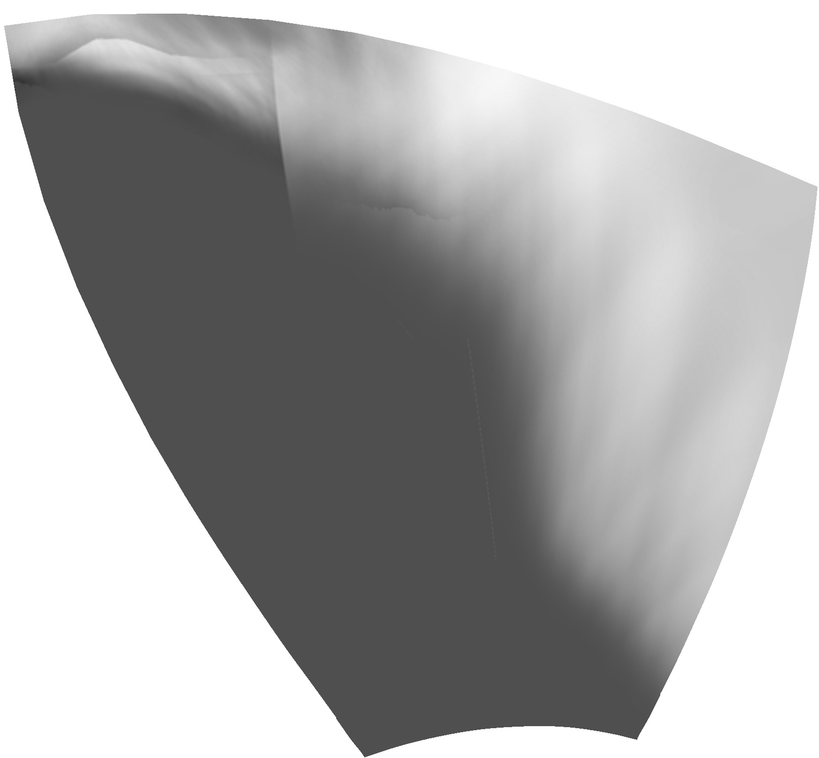
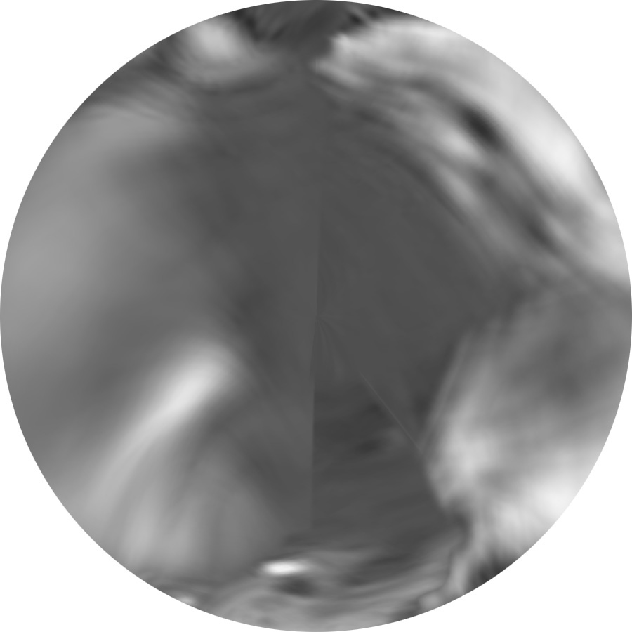
This Borrelly map makes use of a tentative coordinate system illustrated by Howington-Kraus et al. (2002). Their illustration was reprojected to a polar azimuthal projection using (somewhat simplified) grid intersections as tie points. Then the same reprojection was performed on the matching DS1 image. Finally the polar projection was transformed to simple cylindrical projection for archiving and further reprojection.
Reference: E. Howington-Kraus, R. Kirk , L. Soderblom, B. Giese, J. Oberst, 2002. USGS AND DLR TOPOGRAPHIC MAPPING OF COMET BORRELLY. International Archive of Photogrammetry and Remote Sensing, XXXIV(4), no. 277. (Symposium on Geospatial Theory, Processing and Applications, Ottawa 2002)
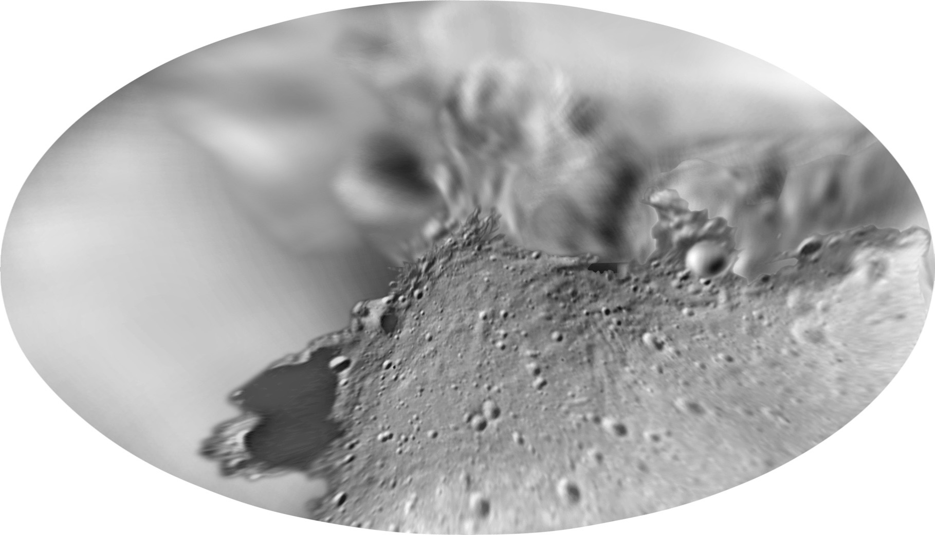
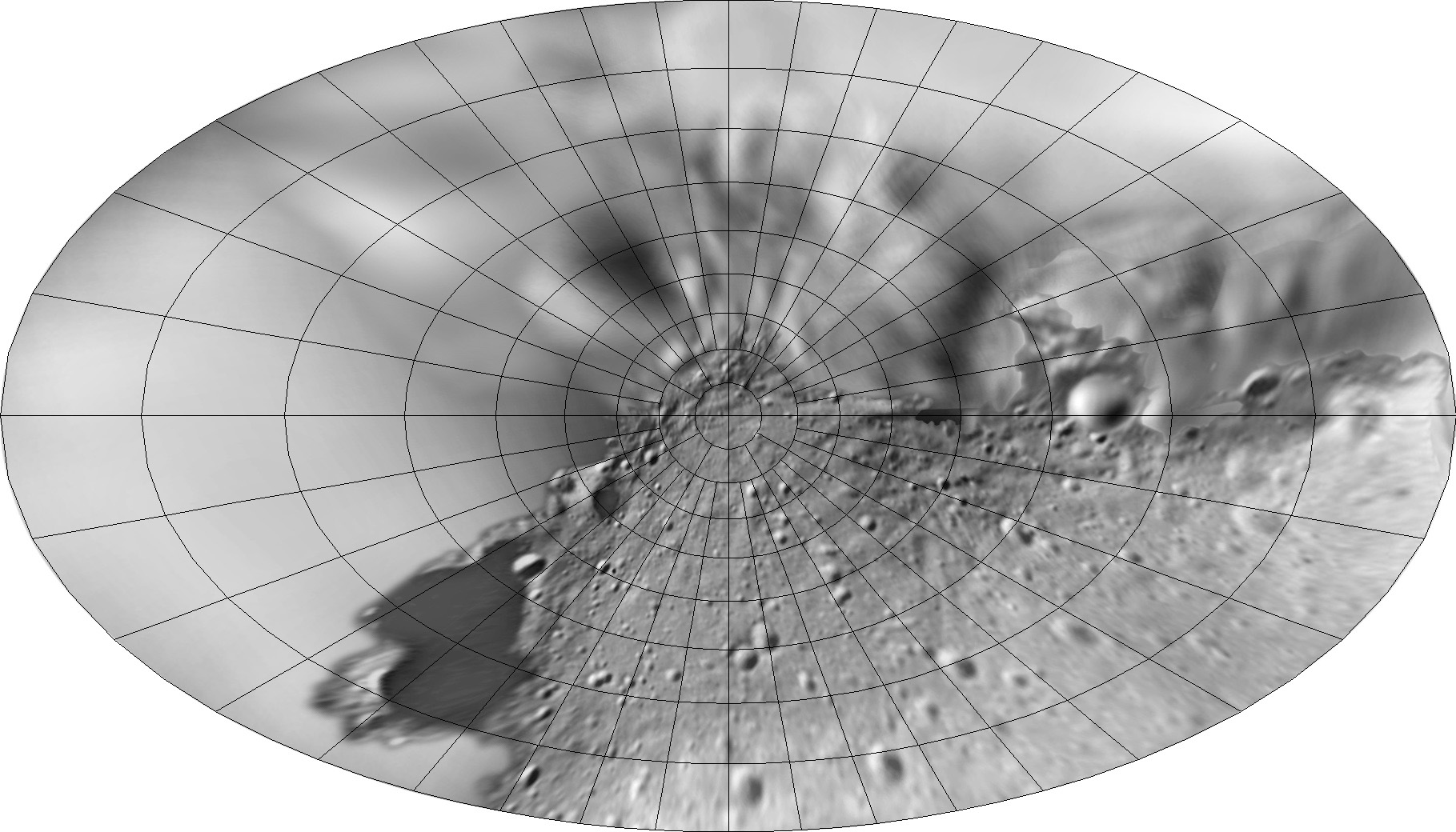
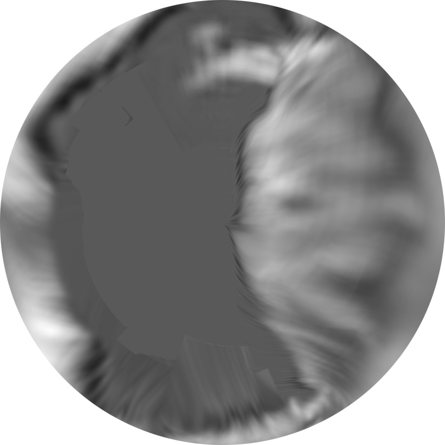
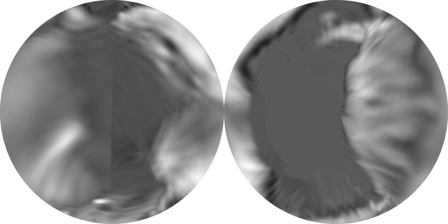
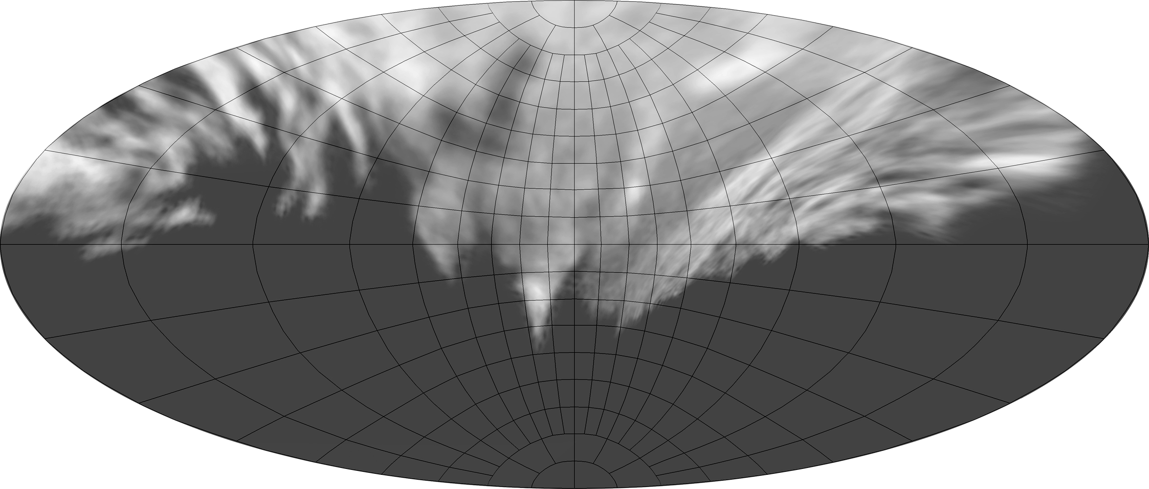
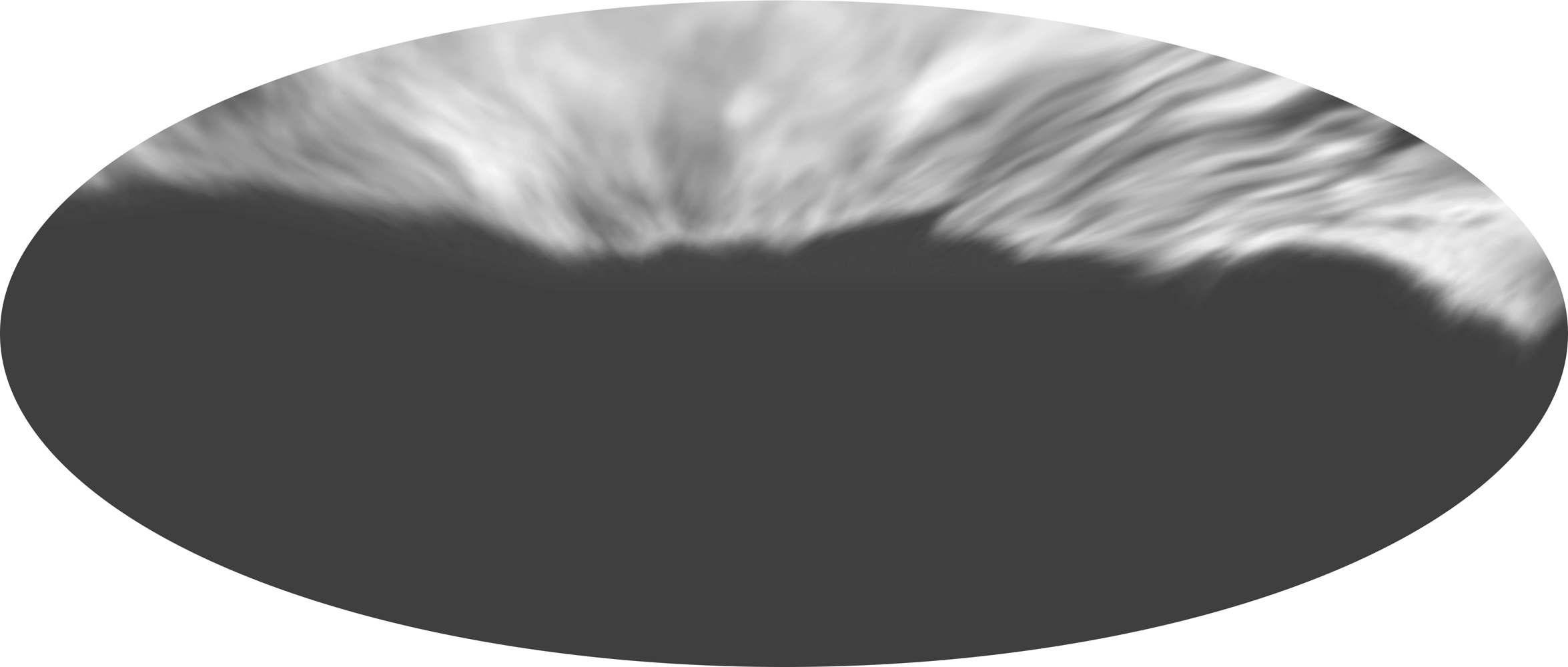
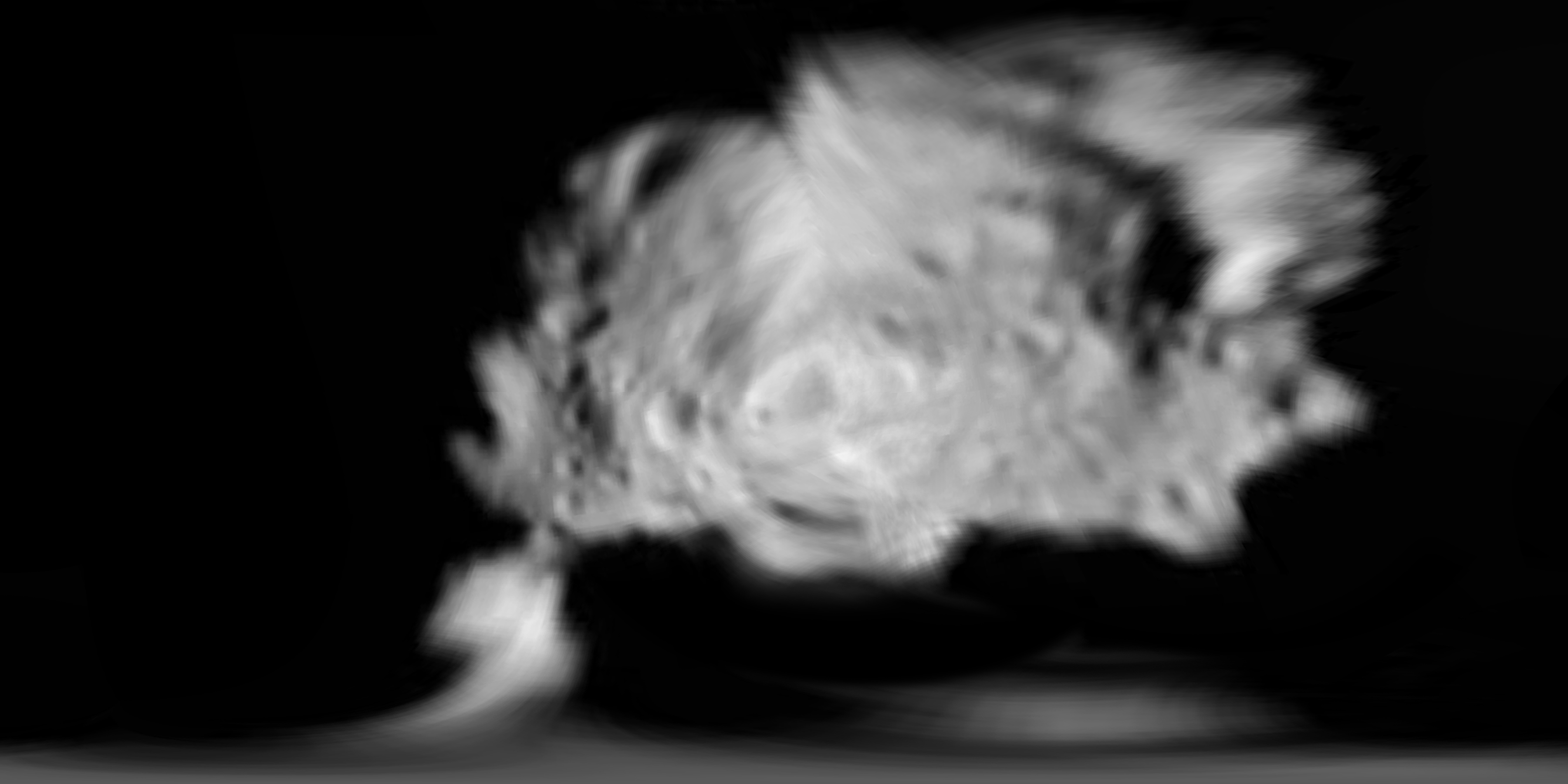
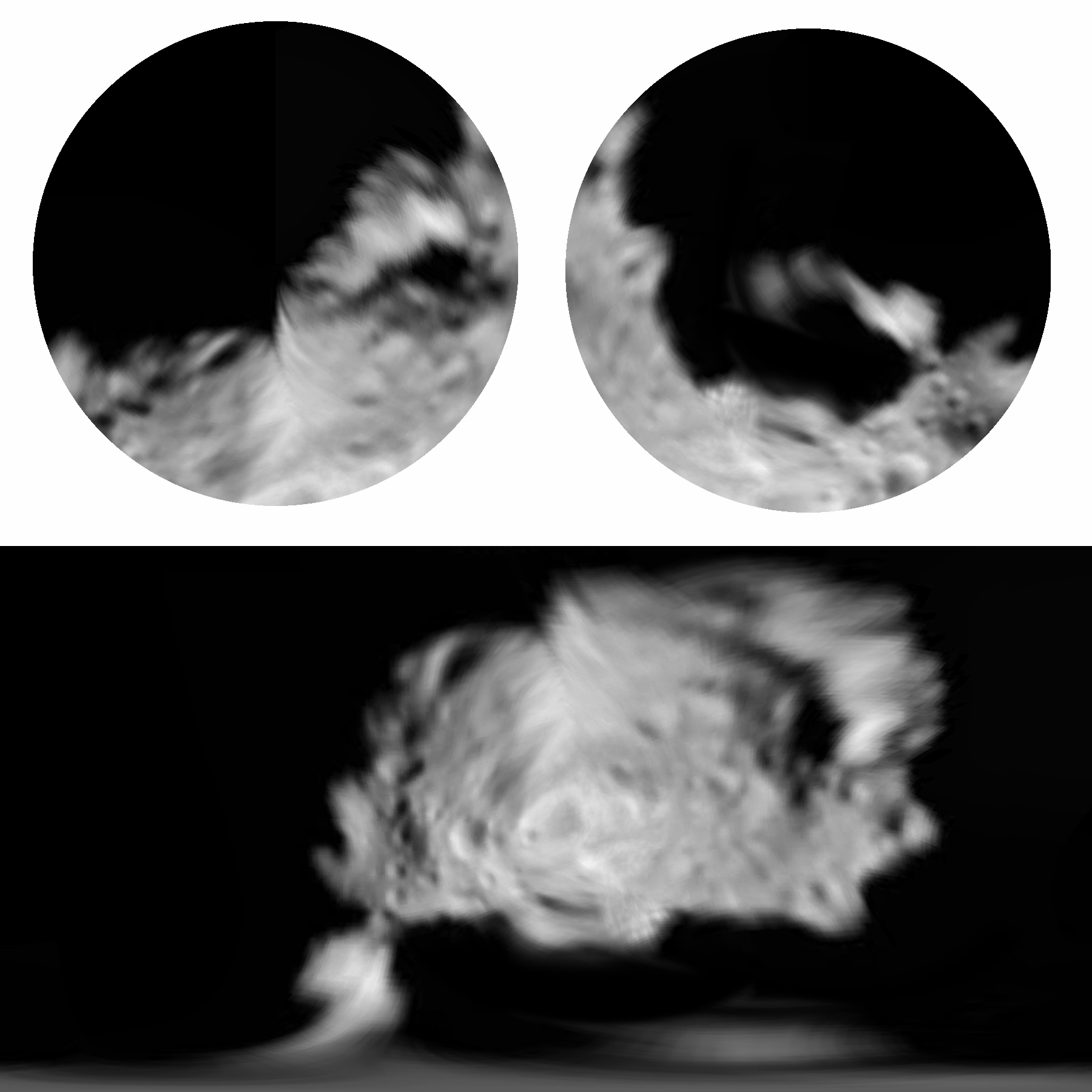
A new mosaic map of the nucleus of Comet Hartley 2. The control is based on maps published by Thomas et al. (2013), the mosaic is a new compilation. Rotation is about the long axis, so the orientation is different from the other ellipse maps. A linear extension into the dark hemisphere toward the southeast (lower right) from the southern hemisphere (north is at top in all maps) locates two very large bocks visible silhouetted against the coma on the limb of the nucleus.
Reference: Thomas, P. C., et al., 2013. Shape, density, and geology of the nucleus of Comet 103P/Hartley 2. Icarus, v. 222, no. 2, pp. 550-558.
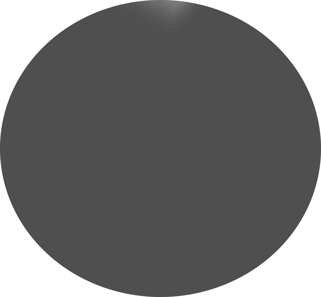
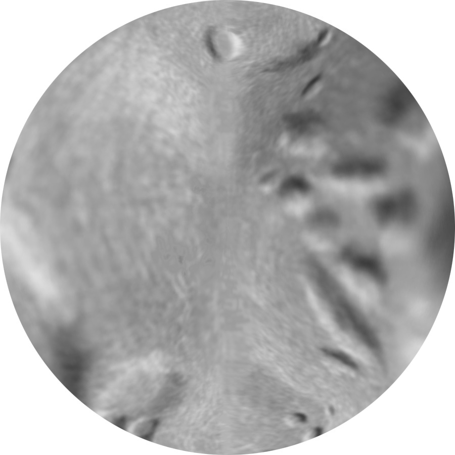
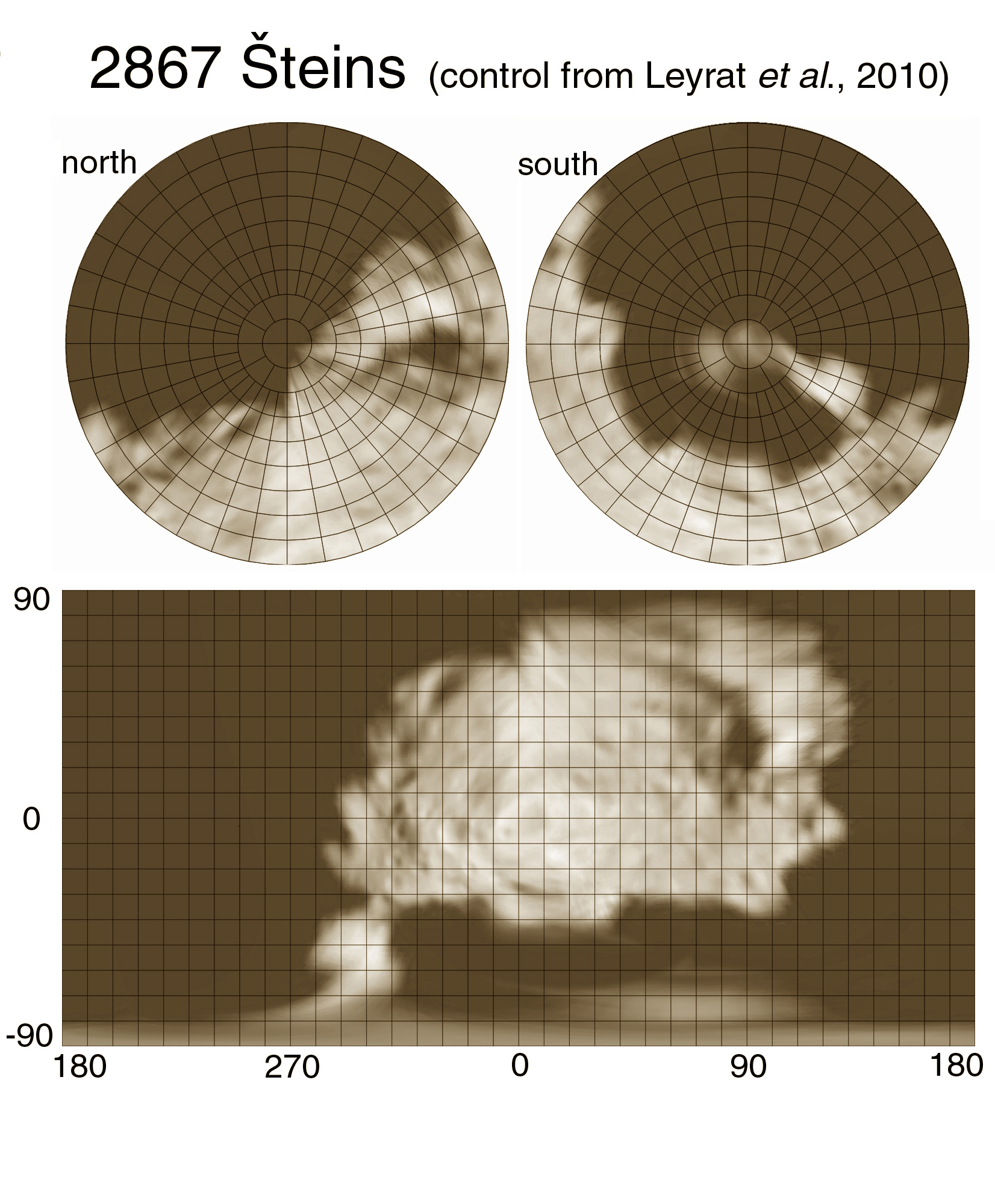
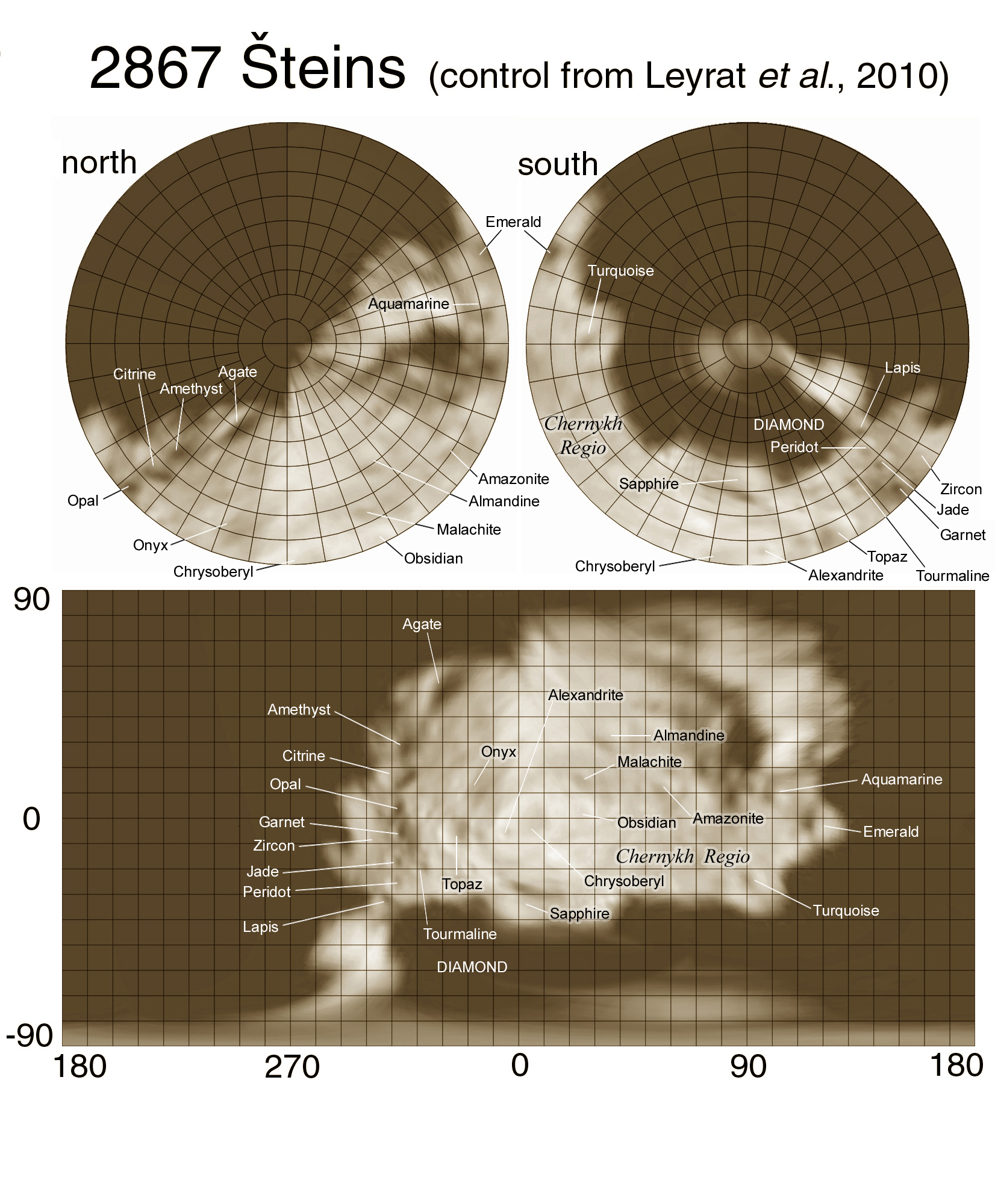
A new mosaic map of Steins. The control is based on a map published by Leyrat et al. (2010). The mosaic is a new compilation, with higher resolution than that by Leyrat and with a different interpretation of the structure of the south pole. The map with feature names is intended to supplement the annotated images at the USGS Planetary Nomenclature website.
Reference: Leyrat, C., et al., 2010. Search for Steins surface inhomogeneities from OSIRIS Rosetta images. Planetary and Space Science, v. 58, no. 9, pp. 1097-1106.