Dawn's Gamma Ray and Neutron Detector:
Ephemeris, Pointing & Geometry at Vesta
T. H. Prettyman
Planetary Science Institute
Part of the Dawn at Vesta Reduced Data Records
Version 1.0, 28-July-2014
Introduction
This document provides an overview of ephemeris, pointing and geometry (EPG) data for the NASA Dawn mission's Gamma Ray and Neutron Detector (GRaND). The data are part of the Planetary Data System (PDS), GRaND Reduced Data Records (RDR) for Vesta Encounter. The data are archived as a single text file. The file contains the position of the Dawn spacecraft in Vesta's fixed frame, the direction to body center in the instrument frame, the solid angle subtended by Vesta at the spacecraft, and ancillary counting and instrument housekeeping data. The information is provided for each science accumulation interval archived in the accompanying Experimental Data Records (EDR, Level 1A). The data can be used for a variety of purposes: for example, selection of data that meet pointing criteria and geometry corrections for counting data. The methods used to determine the quantities recorded in the EPG table are described here.
Identifying Science Data Records across EDR and RDR Files
The Spacecraft Clock (SCLK) value in the science telemetry marks the end of the science accumulation interval with 1s precision. SCLK is a 9 digit unsigned integer that accompanies each science data record in the EPG table. For all GRaND L1A and L1B time series science data files, each record is tagged with SCLK. No two science data records have the same value of SCLK; so, SCLK can be used as a serial number to identify the same science data record in different files. For example, suppose a user has determined the counts in the high energy gamma ray (HEGR) window of the BGO gamma ray spectrum (see Peplowski et al., 2013) for a particular science data record. To determine live time or solid angle for that accumulation interval, the user should search by SCLK for the same record in the EPG table, which contains live time. The true counting rate can be determined by dividing the HEGR counts by live time.
Which Housekeeping Packets Belong to a Science Data Record?
During Vesta encounter, state-of-health (SOH) data were sampled at regular 35s intervals. The SOH data include instrument settings, readings (temperatures and voltages), and scaler counts. The science accumulation interval (TELREADOUT), over which counting data and spectra are accrued, is always selected to be a multiple of the SOH interval (TELSOH). In addition, the SOH sampling always starts 20s before the start of the first science accumulation interval. Two values of TELREADOUT were used during Vesta encounter: 210s when Dawn was far from Vesta; and 70s when Dawn was closer in. For the 210s interval six SOH samples are taken at 15s, 50s, 85s, 120s, 155s, 190s (e.g. see Fig. 1). For the 70s interval, two SOH samples are taken at 15s and 50s. The scalers are reset at the beginning of each science accumulation interval, such that a regular sawtooth pattern can be seen when packets are plotted in sequence.
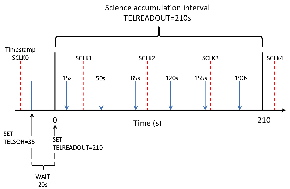
Figure 1. Illustration of how SOH samples (blue arrows) are distributed within a science accumulation intervals. Because TELREADOUT is a multiple of TELSOH, all science accumulation intervals are sampled in exactly the same way. The command sequence (SET TELSOH, WAIT, SET TELREADOUT) determines the time of each SOH sample within the accumulation interval. SOH packets are tagged with the latest value of SCLK from a timestamp command issued by the spacecraft every 60s (red dotted lines). The SCLK value reported for each science data record marks the end of the science accumulation interval with 1s accuracy.
Unfortunately, the SCLK value assigned to each SOH record is inaccurate. Each SOH record is assigned a SCLK value that is updated (via the command telemetry) every 60s (Fig. 1). Thus, two SOH successive packets can have exactly the same SCLK value. So, SCLK alone is not useful for ordering SOH packets.
To reliably determine which SOH packets belong to a science accumulation interval, a quirk in GRaND's software is exploited. Namely, the value of the totals scaler for the last SOH sample within an accumulation interval is repeated in the science data record. All other scalers are properly updated at the end of the science accumulation interval. Whether by accident or design, this peculiar feature is very useful in identifying the last packets in the SOH telemetry that belongs to a particular science accumulation interval. The other SOH packets can be identified using the packet sequence counter. A method to identify SOH packets that sample a selected science accumulation interval is illustrated in Fig. 2.
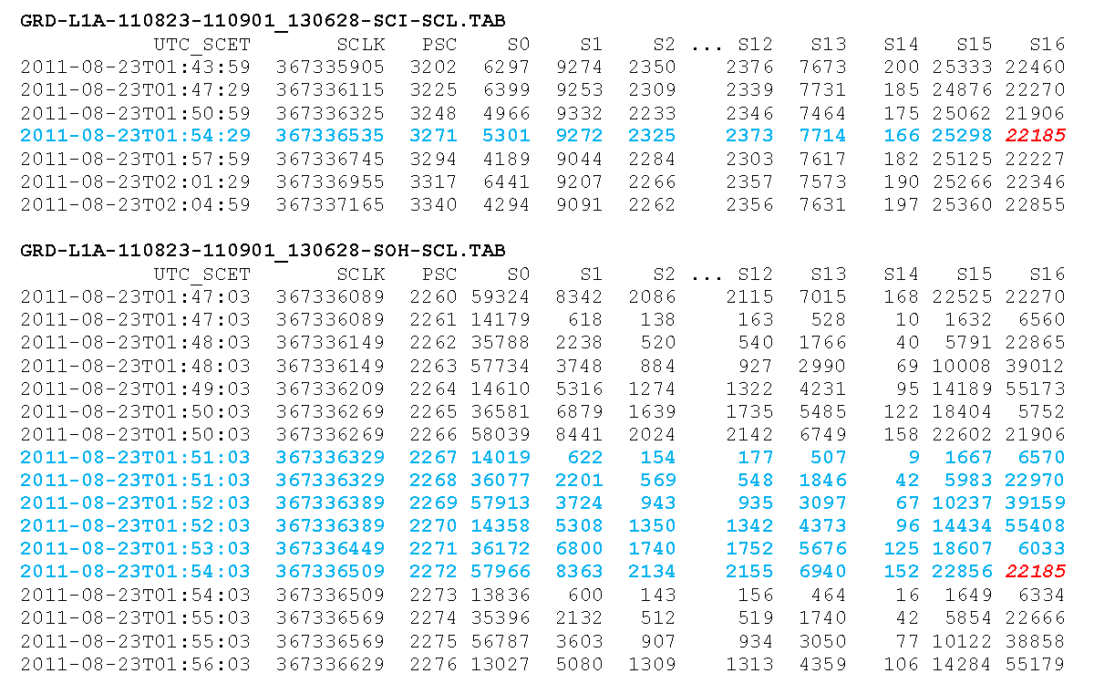
Figure 2. Some SOH and science scaler tables from the PDS archive for Vesta encounter (found in the LEVEL1A_AUX directory of 110811_SURVEY\GRD-L1A-110823-110901_130628). Some of the columns have been expunged for presentation. A science data record is highlighted in the SCI-SCL table (blue). To find out which SOH packets correspond to this science accumulation interval, look for entries in the SOH-SCL table with UTC_SCET and SCLK less than the times listed for the corresponding science data record. Of these, find the latest entry for which S16 (totals scaler) is the same as that of the science data record (marked red/italic in both tables). This is the last SOH sample for the science data record (at 190s). Now, look at the packet sequence counter (PSC) in the SOH-SCL table and count backward to find the other five packets (marked blue/bold). When the PSC is ordered, this algorithm will identify the correct SOH packets.
Counting Data
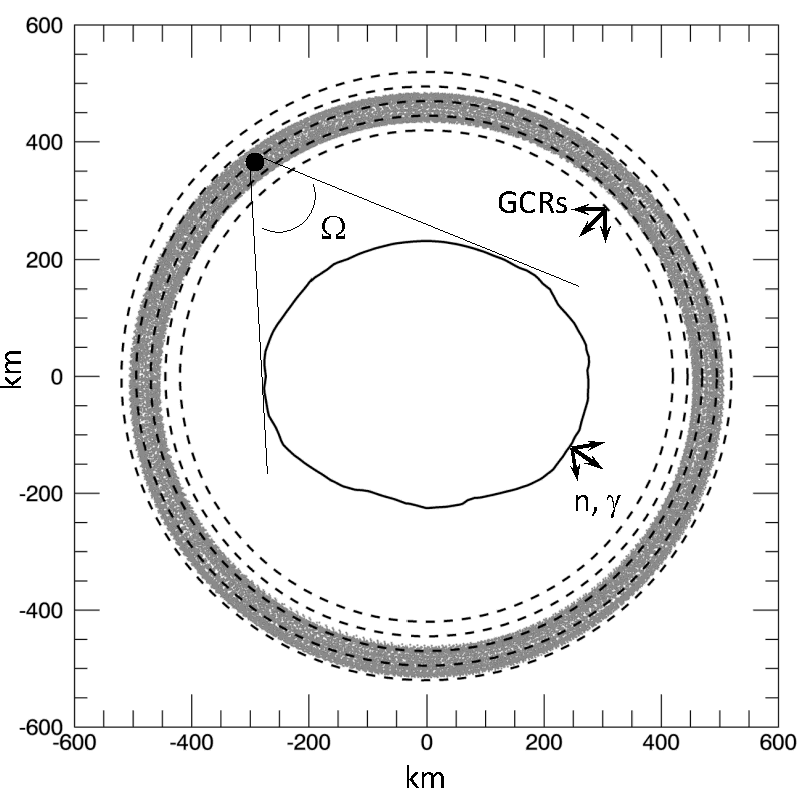
The EPG variations in the flux of galactic cosmic rays. the accumulation time (TELREADOUT) rate (TRIPLES_RATE) are reported. (TRIPLES) incident on the spacecraft (Prettyman et al., 2011) for variations in gamma ray and neutron production in Vesta's surface ( et al., 2013; Peplowski et al., 2013; Yamashita et al., 2013). TRIPLES_ effective accumulation time, known as the "live time." The EPG files contain information needed to determine counting rates corrected for variations in the flux of galactic cosmic rays. For each science data record, the accumulation time (TELREADOUT), live time, and triples-and-higher counting rate (TRIPLES_RATE) are reported. The greater-than-three-sensor-coincidence (TRIPLES) scaler responds to variations in the flux of galactic cosmic rays incident on the spacecraft (Prettyman et al., 2011) and can be used to correct for variations in gamma ray and neutron production in Vesta's surface (e.g. see Prettyman et al. 2011; Prettyman et al., 2012; Prettyman et al., 2013; Lawrence et al., 2013; Peplowski et al., 2013; Yamashita et al., 2013). TRIPLES_RATE is determined for each accumulation interval by dividing counts by the effective accumulation time, known as the "live time." This time is different from the length of the accumulation interval (TELREADOUT).
Each event processed by GRaND takes a finite amount of time to process, during which GRaND is insensitive to new events. Due to the random nature of radiation counting experiments, GRaND could be processing an event when a second event arrives (e.g. a fast neutron event followed immediately by a cosmic ray interaction). In this case, the second event will not be analyzed. Thus, dividing counts by TELREADOUT underestimates the rate at which events occur. The amount of time that GRaND is busy processing events is called the "dead time." While an event is being processed, GRaND counts cycles of a 5 MHz clock using a 26-bit scaler. Only the upper 16 bits are recorded. Thus, each count occurs every 210 (1024) clock cycles. At 5 MHz, the amount of time required to accrue 1024 counts is 204.8 microseconds. The total amount of time GRaND was unavailable to process events (the dead time) can be determined by multiplying the counts accrued over the science accumulation interval by 204.8 microseconds (Prettyman et al., 2011). The true counting rate for any counting product (e.g. gamma ray peak area, region of interest, scaler counts) can be determined by dividing counts by the live time, which is given by subtracting the dead time from TELREADOUT.
A complicating factor is that depending on the length of the accumulation interval, the scaler may roll over one or more times. If this happens, then the dead time counts recorded in the science telemetry at the end of each science interval are low by N x 216, where N is the number of times the dead time scaler rolled over.
For quiet Sun conditions, the dead time counter typically rolls over twice during a 210s interval. For the short accumulation time (70s), the dead time counter usually does not roll over at all; however, during a solar energetic particle event, the dead time counter may roll over many times. GRaND does not count the number of overflow events. Consequently, the number of times a scaler rolls over must be determined in post-processing. Two methods to detect and count roll-over have been explored: 1) analysis of sampled dead time counts within each science accumulation interval; 2) observation of discontinuities in counting rates as a function of time. The former is very effective during quiet Sun conditions; the latter is the only way to determine live time during solar energetic particle events. Both methods have been implemented and tested; however, since the quiet Sun data are most useful for compositional studies, the former method was used in the production of this data set.
Rollover of the dead time counter (scaler S0 in Fig. 2) can be observed in the SOH and SCI data shown in Fig. 2. The progression of counts for the selected accumulation interval is 12019, 36077, 57913, 14358, 36172, 57966, and 5301, where instances of rollover are marked in red. The last value in the sequence is the dead time counter at the end of the science interval. The counter has rolled over twice. Thus, the true value for dead time counts for the selected accumulation interval was 5301 + 2 x 216 = 136373 (27.9s dead time, 182.1s live time). To double check this, take the difference between any one of the monotonically increasing steps in the SOH telemetry that corresponds to a full 35s interval (e.g. 57966 - 36172 = 21794/35s). If counts accrued at this rate, there should have been 130764 counts by the end of the 210s interval (close to, but slightly lower than the counts determined using the rollover algorithm).
The counts projected in this manner are lower than determined by the algorithm due to high dead time at the beginning of the accumulation interval. For example, samples of the dead time count rate in the interior and end of the accumulation interval,
( 36077 - 14019 )/35s = 630/s, ( 36172 - 14358 )/35s = 623s, ( 57966 - 36172 )/35s = 663/s, ( 216 - 57966 + 5301 )/20s = 642/s,
are significantly lower than the dead time count rate at the beginning of the interval 14019/15s = 935/s. We expect that GRaND is busy preparing and transmitting the science data record for a brief period of time following the end of the last interval. Let's assume the instrument is entirely dead for t seconds, after which dead time accrues with a nominal rate of 640/s. If so, then the total dead time counts at the end of the interval is given by
136373 = t/204.8 x 10-6 + (210s -t) x 640/s
This gives about 0.5s ( t = 0.47s ) overhead for preparing and transmitting a science data record.
Temperature Data
GRaND has several internal temperature sensors (Prettyman et al., 2011). Calibrated readings from these sensors can be found in the L1A data set SOH telemetry (-RDG files). The L1B, EPG data file includes readings for the sensor positioned close to the BGO crystal, representative of GRaND sensor head internal temperatures. The temperature readings (T_BGO, given in degrees Celsius) can be used to determine if the instrument internal temperatures have stabilized following power on and high voltage ramp-up. For each science accumulation interval, T_BGO is determined as the average of temperature readings for the associated SOH samples.
Note that the thermistors on GRaND are read out by an 8-bit ADC (Prettyman et al., 2011). The data numbers are then converted to temperature using a linear calibration. Even though the temperatures are represented as a floating point number, they are very coarsely quantitized. For cases in which TELREADOUT=70s, only two SOH samples were available per reading, and a pattern of discrete temperatures is evident in the science-accumulation-interval averages (see Fig. 3). Furthermore, the BGO sensor is thermally well isolated from the interface and has a very long time constant (on the order of 24 hours) Thus, large point-to-point variations (seen in Fig. 3) are likely due to jitter in the reading, rather than actual temperature variations. For studies requiring precise temperatures, smoothing of the data set may be required.
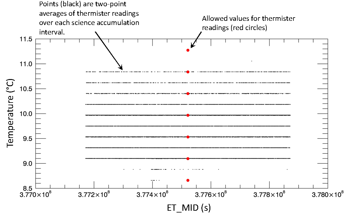
Figure 3. Time series of temperature readings from the thermistor positioned near the BGO sensor (T_BGO). Each point (black dot) is the average of two SOH samples during a 70s science accumulation interval. Each point corresponds to a unique time. The mean of the time series is about 9.5°C. The allowed values for individual samples of the thermistor are shown as red circles. The thermistor was read out by an 8-bit ADC and converted to temperature (degrees Celsius) using a linear calibration ( T_BGO = 0.4354 DN - 32.267 ). The two-point average naturally produces values between allowed thermistor readings.
Instrument Ephemerides and Pointing
The Navigation and Ancillary Information Facility (NAIF) SPICE Toolkit for IDL (version N65) was used to determine spacecraft ephemerides and pointing from the SCLK ticks recorded at the end of each science data record. SPICE kernels for Vesta encounter were downloaded from the NASA Planetary Data System ( http://naif.jpl.nasa.gov/naif/data_archived.html ), dawnsp_1000).
The planetary constants kernel for Vesta (dawn_vesta_v04.tpc) for the Claudia coordinate system was modified with the latest pole position, per private communication by R. Gaskell. The modified PCK file (dawn_vesta_v04b.tpc) can be found in the EXTRAS directory and contains the following:
BODY2000004_POLE_RA  = ( 309.03312     0.0        0.0 )
BODY2000004_POLE_DEC = ( 42.22623      0.0        0.0 )
BODY2000004_PM       = ( 74.6625    1617.3331237  0.0 )
The motivation for using the nonstandard, Claudia system was that the most complete and accurate shape model, used to calculate solid angle (next section) was defined in the Claudia system. Thus, our strategy was to carry out our calculations in Claudia and rotate positions into the International Astronomical Union Claudia Double Prime (CDP) coordinate system for the PDS archive.
For each science data record, the following quantities were calculated:
- SCET_UTC                Spacecraft event time determined from the SCLK value
                           recorded at the end of the science accumulation
                           interval (accurate to 1s);
- ET_MID                  Ephemeris time (s) evaluated at the middle of the
                           science accumulation interval (all values that follow
                           are at the center point);
- PHASE                   The acronym for the mission phase (e.g. "VSL" - Vesta
                           Science LAMO) was determined from the table provided
                           in the mission.cat file, which accompanies this
                           archive;
- LON_C, LAT_C            Longitude and latitude (degrees) of the spacecraft
                           in Claudia coordinate system (DAWN relative to
                           VESTA_FIXED frame);
- POS_XC, POS_YC, POS_ZC  Dawn spacecraft cartesian position in Claudia
                           VESTA_FIXED frame (km);
- DIST                    Distance from the spacecraft to body center;
- DIR_U, DIR_V, DIR_W     Direction of body center in the spacecraft frame
                           (GRaND's frame is identical to that of the
                           spacecraft, see grand_instrument.cat, part of the
                           PDS L1A archive). U, V, and W refer to the X-, Y-,
                           and Z-direction cosines in the spacecraft's
                           coordinate system.
The Claudia coordinates were then rotated into the IAU CDP frame (LON, LAT, POS_X, POS_Y, POS_Z) as follows:
  LON   =   LON_C - 210 degrees; WHERE LON < -180 degrees, LON=LON+360 degrees
  PHI   =   arc_tangent( POS_YC, POS_XC )
  W     =   POS_ZC / DIST
  GAMMA =   SQRT ( 1 - W^2 )
  POS_X =   GAMMA * cosine( PHI )
  POS_Y =   GAMMA & sine ( PHI )
  POS_Z =   POS_ZC
Note that PHI and W are intermediate variables, not reported in the archive. The ephemeris and pointing values were validated by Dr. Steven Joy of the UCLA Dawn Science Center using NASA's Science Opportunity Analyzer (SOA).
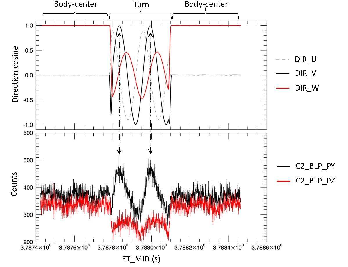
Figure 4. Direction cosines calculated by SPICE are compared with counts measured by GRaND during a portion of LAMO containing a turn to Earth. Before and after the turn, the spacecraft was pointed towards Vesta body center (DIR_U=DIR_V=0, DIR_W=1) for science data acquisition. The turn sampled a range of angles, including instances where the +Y scintillator was facing Vesta (DIR_V=1). When DIR_V=1, the maximum counts for the +Y scintillator (C2_BLP_PY) were observed (as shown by the interconnecting arrows). Similarly, when DIR_W=1, the maximum counts for the +Z scintillator (C2_BLP_PZ) were observed; This happens while body center pointing, not during the turn. The counting data shown are the sum of the Category 2 (C2) BLP-BGO coincidence spectra (BLP component) for the +Y and +Z scintillators. Low-amplitude "wiggles" in counts that can be seen while pointing towards body center result from changes in measurement geometry due to the irregular shape of Vesta.
Pointing can also be validated using GRaND counting data. GRaND +Z and +Y boron-loaded plastic (BLP) scintillators have a mostly-unobstructed, 2π view of space. These outboard scintillators have a cosine-law variation for their response to radiation as a function of direction (Prettyman et al., 2011). The highest counting rates are observed when radiation is incident perpendicular to their surfaces. During Low Altitude Mapping Orbit (LAMO), these sensors respond to the geometry of Vesta (solid angle) and orientation of the spacecraft. For the +Y scintillator, the highest counting rate is expected when Vesta is located in the +Y direction (DIR_U = 1). For the +Z scintillator, the highest count rate is expected when Vesta is in the +Z direction (DIR_W = 1). Low counting rates are expected for (DIR_U or DIR_V < 0), which includes instances where instrument and spacecraft materials intervene between the sensors and Vesta. Fig. 4 shows that the variation of counts measured for the +Y and +Z sensors during science data acquisition and turns to Earth are consistent with the pointing data. The strong changes in counts with direction demonstrates that GRaND is sensitive to radiation originating from Vesta. Wiggles in the counting data during periods of steady, body-center pointing are mostly driven by variations in measurement geometry.
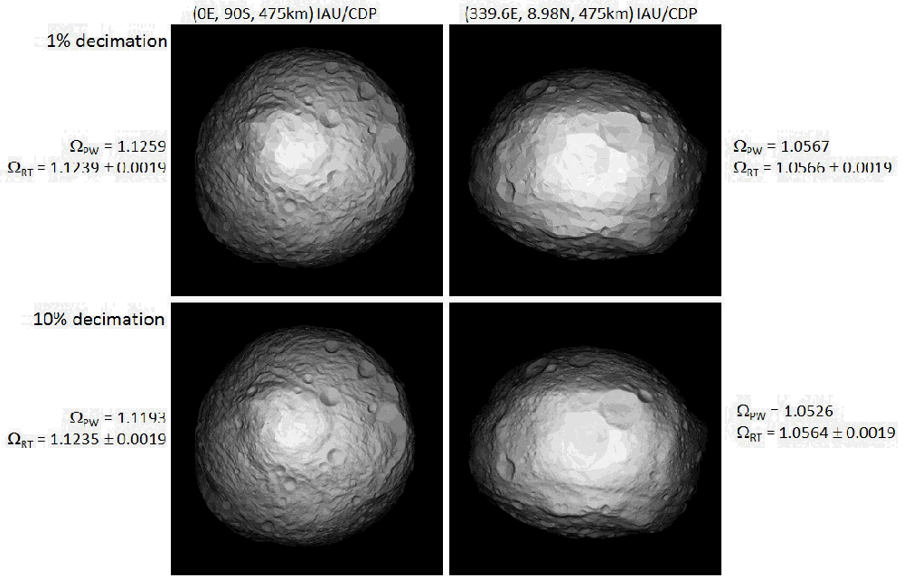
Figure 5. Solid angles calculated by PLATE_WEIGHTS (WPW) and a Monte Carlo ray tracing algorithm (WRT), both with units of steradians, are shown for two locations in the International Astronomical Union Claudia Double Prime coordinate system (IAU/CDP). The images are produced by PLATE_WEIGHTS. The two images on the top are for a shape model decimated to 1% of the original triangles. This model was used to produce the archived data. The images below are for 10% decimation (a much finer scale shape model). The Monte Carlo model is expected to be very accurate, and can be regarded as "truth." Note that the solid angle calculated by Monte Carlo does not vary with decimation. Thus, the coarse (1%) model is adequate for the purpose of calculating solid angle.
Solid Angle - Method and Validation
The solid angle subtended by Vesta at the spacecraft was calculated for the center position of each science accumulation interval using the fast, approximate algorithm described by Prettyman et al. (2011). The fast algorithm uses projective geometry computer graphics to form a 2D image that when summed gives the solid angle. The IDL routine that carries out this task is called PLATE_WEIGHTS. The shape model for Vesta was derived from a Digital Terrain Model provided by the dawn navigation team (GASKELL_CLAUDIA_2014_05_13). The interconnected quadrilateral (ICQ) format was converted to a triangle-vertex model, which was decimated, retaining 1% of the triangles. The decimated shape model used in the solid angle and altitude calculations is provided in the EXTRAS directory in STereoLithography (STL) format (binary) and as a Type 1 triangle vertex file (ASCII).
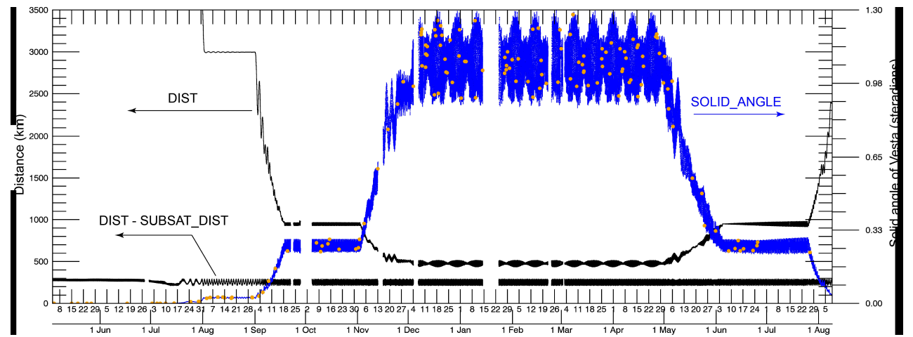
Figure 6. Survey of all data acquired during Vesta encounter. The distance to body center (DIST, km), and distance from Vesta body center to the surface of the shape model in the direction of the spacecraft ( DIST - SUBSAT_DIST, km ), and the solid angle subtended by Vesta at the spacecraft ( SOLID_ANGLE, steradians )are shown. Orange points are SOLID_ANGLE values randomly sampled from the data set for comparing results of PLATE_WEIGHTS and Monte Carlo ray tracing (see Fig. 7).
The solid angle calculation was validated using a Monte Carlo, ray-tracing algorithm. For an isotropic source of rays located at the spacecraft, the solid angle is the ratio of the number of rays striking the shape model to the total number of rays sampled multiplied by 4π. The calculation can be accelerated by sampling only those rays that head in the direction of a sphere bounding the shape model. Using this simple, problem-truncation method for variance reduction, the solid angle can be determined accurately and precisely for distances very far from Vesta in a reasonable amount of time. The shape model ray intersection algorithm was also used to determine the distance to Vesta's surface in the nadir direction (SUBSAT_DIST).
A comparison between the fast algorithm and the Monte Carlo method is shown in Fig. 5. The 2D images show the output of PLATE_WEIGHTS (PW). The solid angle calculated by PLATE_WEIGHTS (WPW) and by ray tracing (WRT, along with the Monte Carlo precision) with units of steradians is shown next to each image. Two spacecraft locations are shown: over the south pole, 475 km from body center (left images); and over the crater Marcia near the equator and at the same distance (right images). The images on the top are for the shape model decimated to 1% polygons, which was used to calculate the solid angles in the archive. The images on the bottom are for a higher resolution shape model (10% decimation). Within the precision of the Monte Carlo calculation, the solid angles calculated for the coarse (1%) and fine (10%) shape models are identical. This shows that the coarse model is adequate for estimating solid angle; refining the resolution of the model beyond 1% does not improve accuracy. The PW approximation, while accurate at both spatial scales, is highest for the coarse model. The accuracy of PW depends in part on the size of the projected image, which was the same for both cases. Nonetheless, the difference between PW and RT is less than 0.5% in the examples shown.
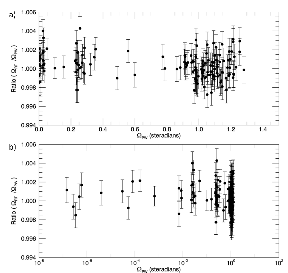
Figure 7. Comparison between calculations of the solid angle by PLATE_WEIGHTS (PW) and Monte Carlo ray tracing (RT) for randomly sampled locations (orange points, Fig. 6).
PW and RT calculations were compared for 150 randomly selected spacecraft positions during Vesta encounter (orange symbols in Fig. 6). The ratio of the solid angle calculated by RT to PW is shown in Figs. 7a and 7b. The abscissa (WRT) was selected to show the full range of solid angles during Vesta encounter. The PW calculation with the 1%-decimated model is accurate to better than 0.5% for all locations tested and the population standard deviation of the ratio ( 0.0013) is consistent with mean uncertainty in the ratio (also 0.0013, given by the average of the error bars in Fig. 7). In summary, the PW estimate of solid angle included in the archive is accurate to within 0.5%, and probably much better.
References
Lawrence D. J., Peplowski P. N., Prettyman T. H., Feldman, W. C., Bazell
D., Mittlefehldt D. W., Reedy R. C., and Yamashita N. 2013. Constraints
on Vesta's elemental composition: Fast neutron measurements by Dawn's
gamma ray and neutron detector. Meteoritics & Planetary Science,
doi:10.1111/maps.12187.

Peplowski P. N., Lawrence D. J., Prettyman T. H., Yamashita N., Bazell D.,
Feldman W. C., and Reedy R. C. 2013. Compositional variability on the surface
of 4 Vesta revealed through GRaND measurements of high-energy gamma rays.
Meteoritics & Planetary Science, doi:10.1111/maps.12176.

Prettyman T. H., Feldman W. C., McSween H. Y. Jr., Dingler, R. D.,
Enemark D. C., Patrick D. E., Storms S. A.,, Hendricks J. S.,
Morgenthaler J. P., Pitman K. M., and Reedy R. C. 2011. Dawn's Gamma Ray
and Neutron Detector. Space Science Reviews 163:371-459.

Prettyman T. H., Mittlefehldt D. W., Yamashita N., Lawrence, D. J.,
Beck A. W., Feldman W. C., McCoy T. J., McSween H. Y., Toplis M. J.,
Titus T. N., Tricarico P., Reedy R. C., Hendricks J. S., Forni O.,
Le Corre L., Li, J.-Y., Mizzon H., Reddy V., Raymond C. A., and
Russell, C. T. 2012. Elemental mapping by Dawn reveals exogenic, H in
Vesta's regolith. Science 338:242-246.

Prettyman, T. H., Mittlefehldt, D. W., Yamashita, N., Beck, A. W., Feldman,
W. C., Hendricks, J. S., Lawrence, D. J., McCoy, T. J., McSween, H. Y.,
Peplowski, P. N., Reedy, R. C., Toplis, M. J., Le Corre, L., Mizzon, H.,
Reddy, V., Titus, T. N., Raymond, C. A., Russell, C. T. 2013. Neutron
absorption constraints on the composition of 4 Vesta. Meteoritics &
Planetary Science, doi: 10.1111/maps.12244.

Yamashita N., Prettyman T. H., Mittlefehldt D. W., Reedy R. C.,
Feldman W. C., Lawrence D. J., Peplowski P. N., McCoy T. J., Beck A. W.,
Toplis M. J., Forni O., Mizzon H., Raymond C. A., and Russell C. T. 2013.
Distribution of iron on Vesta. Meteoritics & Planetary Science,
doi:10. 1111/maps.12139.