------------------------------------------------------------------------------
prepared by: S.E. Schröder (signature/date)


------------------------------------------------------------------------------
approved by: A. Nathues (signature/date)
   ===========================================================================
   Iss./Rev.      Date    Pages affected   Description
   ===========================================================================
   Draft      21/01/2009      All          first draft

   D/1        28/01/2009                   minor changes to §3, added Figure 1

   1/�        29/01/2009                   rearranged Figures and Tables, edited Figure 1.

   2/�        28/06/2011                   Edited §1.2, §2.1, §2.3-§2.7, revised §2.8.
                                           Edited Figs. 1, 2, 3, 9, deleted Figs. 4, 12,
                                           exchanged Fig. 11. Added Figs. 5
                                           and 13. Updated Table 2, revised Table 3.
                                           Deleted §4. Various small changes through�out the text.

   2/a        20/07/2011                   Corrected Eqs. 7, 8, 9.

   2/b        2013-10-22      All          Replaced the expression "hot pixels"
                                           with warm pixels
                              2-3          Removed Approval Sheet and Distribution
                                           Record
                              Section 1    Removed reference documents
                              Section 2.5  Updated flat field correction algorithm
                              Section 2.7  Commented on the difference between bad
                                           and warm pixels
   ===========================================================================
1������� General Aspects...................................................... 6
1.1�������� Scope............................................................. 6
1.2�������� Introduction...................................................... 6
2������� Calibration Overview................................................. 7
2.1�������� Bias.............................................................. 7
2.2�������� Residual charge................................................... 8
2.3�������� Dark current...................................................... 8
2.4�������� Readout smear.................................................... 10
2.5�������� Flat fields...................................................... 10
2.6�������� Radiometric calibration.......................................... 11
2.7�������� Bad pixels....................................................... 13
2.8�������� Geometric distortion............................................. 14
3������� Pipeline Architecture............................................... 26
3.1�������� Executable architecture.......................................... 26
3.2�������� Configuration file............................................... 27
Figure 1. Layout of a full frame image (to scale). The active area is displayed in light blue, the optically shielded regions in dark blue, and the pre- and post-scan regions in red (note that these are not physically part of the CCD). Area size is indicated in (columns x rows). The coordinates of the pixels in the lower left and upper right corner of the full frame are (0,0) and (1091,1055), respectively. The coordinates of the pixels in the lower left and upper right corner of the active area are (34,16) and (1057,1039). When we consider the active area only, we refer to these pixels as having coordinates (0,0) and (1023,1023). The storage area is located below the area shown here. The horizontal (read-out) direction is referred to as the sample- or x-direction, the vertical direction is the line- or y-direction, consistent with the definitions in the SPICE kernels.
Figure 2. The bias of FC1 images acquired during the ICO Performance and Calibration blocks compared to the CCD temperature. Left: FC1, right: FC2.
Figure 3. Pre- and post-launch dark current in [DN/sec] of a typical CCD pixel, calculated as the mean of row 1000. The post-launch data (ICO/MGA) represent 300 [s] exposures only. The lines are fits of the model in Eq. 1 through the pre- and post-launch data (dashed and dotted lines, respectively). Post-launch data are corrected for warm pixels and cosmic rays.
Figure 4. FC2 dark current evolution over the course of the 9 days from the ICO Performance to the Calibration blocks . New warm pixels are located in the horizontal branch at the bottom.
Figure 5. The de-smear algorithm in action. The FC1 observed an illuminated pinhole through a collimator through F1 (8 Mar 2006). Exposure time was 60 [ms]. Left: original image (average of two). Right: image after de-smearing. The brightness is scaled identically in both, such that black and white are equivalent to �5 DN and 30 DN, respectively. The peak signal in the central spot was 13110 DN. Note that a weak ghost is visible at the right of each image.
Figure 6. The normalized flat fields of FC1 (left) and FC2 (right). Brightness is scaled such that values <0.90 are displayed as black, and values >1.05 as white. A faint diagonal pattern is due to stray light associated with the experimental setup.
Figure 7. Diagonal profiles through the flat fields in Figure 6, running from pixel [0,0] to [1023,1023]. The profiles have been subjected to a 7-pixel wide median filter.
Figure 8. The FC1 absolute responsivity for the different filters as determined from the lab calibration.
Figure 9. The measured flux of a point source (in this case Vega observed by FC1 through F7) depends strongly on the position of the PSF on the pixel, especially in x-direction because of the presence of anti-blooming gates. The x-axis denotes the distance of the center of the PSF to the center of a pixel, as determined by a 2D Gaussian fit.
Figure 10. The flux of three photometric standard stars observed by FC1 (left) and FC2 (right) for all filters compared to that expected if the lab calibration in Figure 8 were correct. The Vega data are the mean and standard deviation of ~10 observations. The 73 Cet and 42Peg data are two single observations per filter.
Figure 11. Verification of the responsivities in Table 2. Left: The solar spectrum (black) fitted to the intensity of solar analog 51 Peg (red triangles), observed during the ICO Calibration block. The intensity was integrated over a 15x15 pixel block surrounding the star. There were two observations in each filter; for clarity, error bars are shown for only one. Right: Reconstructed intensity coming from the Martian surface for F5 image 1010, acquired during MGA. The plot compares the reconstructed intensity (red bullet; calculated with the F5 responsivity in Table 2) to that expected for the ubiquitous bright red soil (black line). The expected spectrum was calculated by scaling the Mars geometric albedo to bright soil BRDF measurements by the Spirit rover for the FC observation phase angle (blue bullets; from Johnson et al. [2006] JGR 111, E02S14).
Figure 12. Investigation of CCD linearity. Shown are the mean FC1 and FC2 charge rates in a 100x100 pixel block in the lower left corner as a function of median charge in lab flat field images (FC1: 24 Feb 2006; FC2: 12 Aug 2005). The FC2 charge rate is normalized to that associated with the lowest median charge. The FC1 charge rates were higher, but scaled to match the FC2 series. Some scatter in the data is due to uncertainties in exposure time.
Figure 13. FC2 geometric distortion characteristics. Left: Focal length as a function of wavelength. Right: The radial distortion parameter k1 depends on wavelength (lateral chromatic aberration). The dashed line is a linear fit to the data.
Figure 14. Flow chart for the calibration pipeline algorithm. 'Callamp' is an image of the inside of the camera cover illuminated by the internal calibration lamp (labeled 'flat field' in the PDS image header).
Table 1. Integrating sphere images averaged for flat field construction. FC1 flat fields were acquired on 24 Feb 2006 (TCCD ~ 230 [K]), FC2 flat fields on 12 Aug 2005 (TCCD ~ 233 [K]).
Table 2. Filter characteristics, absolute responsivity, and effective solar flux for both cameras and all filters. lcen and leff are the filter band center and effective wavelength, respectively, in [nm]. The radiance is obtained by dividing the pixel signal (in DN / sec) by R. The result of this division has units as indicated in the rightmost column.
Table 3. Geometric distortion characteristics of each filter (focal length f, radial distortion parameter k1, and the IFOV), found by fitting ~100 star positions in ICO Performance (FC1 and FC2) and DC041 (FC2 only) images of the field around 20 Cep (p1 = p2 = 0).
This document describes the pipeline for calibration of the images acquired by both models of the DAWN Framing Camera (FC1 and FC2). It details its operation and implementation. The pipeline builds on the results of the analysis of in-flight [1] and laboratory measurements [2-5]. This document presents the pipeline in its current state, and will be updated when necessary.
We have developed a pipeline for calibrating FC science images. It is based on lab measurements and in-flight data acquired during the Initial Checkout Operations (ICO) and the Mars Gravity Assist (MGA). ICO was divided into three observation blocks: Functionality, Performance, and Calibration. The results of observations of calibration targets like star fields and photometric standard stars during Performance and Calibration have been incorporated in the pipeline. Section 2 describes in detail how we calibrate the images, and which data (lab/ICO) have been selected for this purpose. The pipeline has been implemented as a stand-alone executable, which is described in Section 3.
Properly calibrating FC images requires a full understanding of the CCD layout. The active area of the Atmel/Thomson TH7888A CCD is sized 1024x1024 pixels or 14.34 x 14.34 [mm2] (14.00x14.00 [µm2] per pixel). Columns and rows surrounding the active area are covered (optically shielded) to be used for diagnostic purposes (e.g. dark current characterization). FC images can be transmitted in as a 1092x1056 pixel sized full frame, that includes these extra regions plus an additional 12 columns at the left and 34 columns at the right of the image [2]. These additional columns, named pre- and post-scan regions, do not represent physical columns of the CCD, but are filled by the output amplifier. If we define (0,0) as the coordinates of the pixel at the bottom left of the full frame image (where an image is read out), then the active area is that enclosed by rows [16:1039] and columns [34:1057] (Figure 1). The covered lines that can be used for dark current characterization are rows [1:12] and [1043:1054] and columns [13:28]. For the remainder of this document the word 'image' refers to the active area only, unless specified otherwise.
After converting the raw 14-bit integer pixel values into floating-point the following steps are applied to calibrate an image:
Step 6 includes division by the exposure time. Concerning step 7: to date, no bad pixels have been identified. Each of the steps is explained in detail in the following paragraphs.
The degree to which images are calibrated is indicated by levels. Level 1a images are the raw images in PDS format that have been extracted (decompressed) from the spacecraft data stream. Level 1b images have been calibrated up to, and including, bad pixel removal (point 7 in the list). In some color filter images the level of in-field-stray light may be relatively high (see §5). It may be possible to correct for this, the result being level 1c images. Level 1d images are level1b (or 1c) images that have been geometrically corrected. Cosmic rays are not removed from the images.
The CCD output amplifier operates at a certain voltage to prevent the occurrence of negative values (due to noise). This effectively adds a certain (ideally identical) value to all pixels in the image that is called the bias. This bias has to be subtracted as the first step in the calibration pipeline. The leftmost 12 columns of the full image frame are known as the pre-scan region. These do not represent a physical area on the CCD, but instead are filled by the output amplifier with bias values. We estimate the bias applied to the image as the average of columns [0:11], and subtract this number from the raw image. By calculating the mean of this area one finds a typical bias uncertainty of 1-2 DN (read-out noise). The typical FC bias is between 250 and 300 DN, with the FC1 bias is slightly higher (~10 DN) than that of FC2. The bias value correlates with CCD temperature (Figure 2), but also with the temperature of other components [7]. Bias values that have been observed in-flight are between 258 and 272 DN for FC2, and between 271 and 283 DN for FC1.
"Bias frames" (zero second exposures) acquired pre-launch show no variability over the frame other than the read-out noise. Zero second exposures are routinely acquired in-flight as part of the semi-annual calibration activity. Apart from the occasional presence of cosmic rays they show no variability over the frame. On average, the data numbers are slightly higher in the active area than in the bias region (the leftmost 12 columns), consistent with accumulation of dark current in the storage area during read-out.
Charge that is present on the CCD before the start of an exposure has been found to affect FC1 [4]. This phenomenon is referred to as residual, or extra charge. It can accumulate while the CCD is illuminated before the exposure starts because the anti-blooming gates do not function properly. The amount of extra charge has been quantified from lab flat field images, and has been found to be a pixel-specific function of the intensity of the light observed and the duration of the pre-exposure [1]. Stellar fluxes are too low to induce the effect, but since neither FC1 nor FC2 has been subjected in the lab to light fluxes as high as will be experienced at Vesta, it is not known how strongly images will be affected during the asteroid encounters. Analysis of FC2 flat field images has not uncovered any evidence for extra charge. However, since lab light exposure levels were rather low, it is expected that Vesta images will show at least some extra charge.
In principle, if the amount of extra charge is known it can be subtracted from the image. In practice this may not be so simple, as it depends on the scene witnessed before the start of the exposure. Our current understanding of the phenomenon is not sufficient yet to develop mitigating measures, but if we are fortunate we may never need these.
The next step in the calibration pipeline is the subtraction of dark current. Let us first compare the FC dark current behavior before and after launch. Pre-launch dark current measurements were acquired on 15 February 2006 (FC1) and 12 August 2005 (FC2). Due to lab hardware limitations these were all obtained at higher temperatures than achieved in-flight. A small fraction of pixels exhibit above-average dark current, and we call these 'warm' pixels. We compare the dark current of regular pixels in Figure 3. Both cameras behave very similar. The in-flight dark current is slightly increased with respect to the pre-launch measurements. Before launch, the CCD had very few warm pixels. For example, only 136 pixels (0.013%) in FC2 image 25508 have a dark current exceeding the mean plus 4σ (calculated for column 10 of the active area). Now that DAWN has launched, the number of warm pixels is increasing steadily with time.
The analysis of in-flight (ICO/MGA) dark current images is hampered by the presence of cosmic rays. At the operational CCD temperatures T ~ 220 [K]) dark current is very low. To accurately measure it we need long exposures, but this also leads to more cosmic ray hits. A good compromise is an exposure time of 300 [s]. We find that dark current typically contributes 10-20 DN in 5 minutes in the in-flight temperature range. A subtle gradient is present across the FC2 CCD, with the dark current at the top around 20% higher than at the bottom.
Figure 4 shows the change in dark current for all pixels over a period of 9 days between the two ICO blocks Performance and Calibration by comparing the associated reference dark frames. The vast majority of pixels are located in the lower left corner of the figure, and have a stable dark current of 0.02-0.06 DN / sec at the reference temperature of Tref = 218 [K]. Warm pixels can be found further up the diagonal. Note that their charge rate is also stable over time. Visible as a horizontal branch are new warm pixels that have appeared within these 9 days. The absence of a vertical branch demonstrates that our cosmic ray filtering technique is effective. From this and similar figures we derive an average warm pixel generation rate of around 27 pixels per day (for both cameras) over the full ICO campaign. The number of warm pixels in the FC2 Calibration reference dark frame (again defined as exceeding the mean plus 4s) has grown to 3392 (0.32%).
We employ a dark current model to calibrate the in-flight images. Each image is corrected for dark current individually by subtracting a dark frame d, which is constructed from a reference dark frame dref. The reference dark frame is built from actual dark exposures acquired close in time to the image to be corrected. The dark current D (in DN / sec) of a typical pixel is assumed to follow the following formula:
where A and B are constants, T in [K] is the CCD temperature, and kB = 1.38065�10�23 [m2 kg s�2 K�1] is the Boltzmann constant. We determine the typical dark current by taking the average of row 1000 of FC dark current exposures, discarding anomalously high values due to warm pixels and cosmic rays. The model fits in Figure 3 reveal that the bulk dark current has increased slightly following launch. From the pre-launch measurements we determine the constant in the exponent as B = 1.018�10�19, which is adopted for all dark current curves. For FC1 we find A = 8.91�1012 (pre-launch) and 1.35�1013 (post- launch), and for FC2 we find A = 1.26�1013 (pre-launch) and 2.03�1013 (post-launch). The reference dark frame dref is constructed as the median over a set of 300 [s] dark exposures that have each been corrected for actual CCD temperature by multiplication with D(Tref) / D(T). The dark frames d used to calibrate the images are a multiple of dref:
The difference between the reference temperature and the CCD temperatures at which science exposures are acquired is typically less than 2K.
In principle, there is another source of dark current for which one can correct. After the image is transferred from the active into the storage area of the CCD it takes 1.159 [s] to be read out. During this period the image acquires dark current. However, at the low CCD temperature of science operations the dark current in the storage area is about half that of the active area [3], hence its contribution to the image would be on the order of 0.03 DN at most. This value is so low that we do not need to correct for it.
Upon finishing an exposure the image is transferred from the exposed region on the CCD downward to the covered storage region for read-out. During this rapid (1.32 [ms]) transfer, the image continues to be exposed. The bottom rows will enter storage directly, but the top rows will accumulate charge all the way down to the storage area, which introduces a gradient from image top to bottom. This is known as the 'electronic shutter effect'. If the exposure times are on the order of the shift time, the image needs to be corrected for this smear.
We have developed an algorithm that calculates the smear from the image content, which implicitly assumes that the scene witnessed during the transfer is precisely that captured by the image. It starts with the fact that it takes exactly 1.320 [ms] to shift all 1056 rows of the full image frame, so the shift time per row is tshift = 1.250 [µs]. Only 1024 rows (active area) are actually exposed for a time texp (in [s]). It iteratively subtracts the image smear by calculating the smear contribution si for row ri as:
We start with calculating the smear s16 for the bottom row of the active area, which is then subtracted from lines r17 to r1055, i.e. all rows above r16. This procedure is then repeated for row r17 (whose content has now changed!), and subsequently to the remaining rows of the active area (r18 to r1039). A successful application of this algorithm is shown in Figure 5.
Before launch both cameras observed the illuminated inside of an integrating sphere on 24 February 2006 (FC1) and 12 August 2005 (FC2). We construct FC flat fields as the average of several individual exposures (Table 1), acquired at similar CCD temperature and each corrected for bias. Because the F8 exposure times were much longer than those of the other filters (>=200 sec versus <3 sec), the F8 flat fields were corrected for dark current (instead of simply for bias) by subtracting an average of three dark frames with identical exposure times acquired at similar temperatures during the same session. The dark current for the other filters can be ignored because of much shorter exposure times. The flat fields are normalized to the average of pixels [579:619, 493:553], which is where the diffused monochromator signal was observed through the collimator during the FC1 radiometric calibration session (see §2.6).
The resulting flat fields for both cameras are displayed in Figure 6. Visible in all are dark circular spots (presumably dust particles on the CCD), a horizontal pattern of stripes (a property of the CCD), and bright blemishes in the F8 flat fields (probably associated with the filter). Apart from these features it appears that the flat fields of some filters are not flat at all, but darkened towards the edges. Both cameras are very similar in this respect. The diagonal profiles in Figure 7 enable a quantitative assessment. The flat field of the clear filter (F1) is flat to within 1%, but that of some color filters (especially F4, F6, F7, and F8) have darker edges and corners, where the brightness is up to 10% lower than in the center. This phenomenon has been traced to an accumulation of in-field stray light in the center of images taken through some color filters when observing an extended target. The same phenomenon seems to affect the Messenger camera, which uses the same CCD [2].
In order to correct for this effect, the flat fields have been processed by means of a convolutional algorithm that removes the in-field stray light. This technique removes the darkening towards the image edges, but preserves dust specks present on the CCD and horizontal striping. We do note, however, that these dust specks may be expected to have moved or disappeared during launch, as has been observed during the FC2 out-of-field stray light test [9].
Some characteristics of the FC filters are listed in Table 2. The central wavelength λcen is defined as the average of the wavelengths that define the FWHM of the filter transmission curve [3]. Prior to launch the responsivity of the cameras as a function of wavelength was determined by observing the output of a monochrometer through a diffuser and collimator [5]. The spectral responsivity ri(λ) for filter i in [J�1] is shown in Figure 8. From this we calculate some filter characteristics as listed in Table 2. We define the filter effective wavelength of filter i as
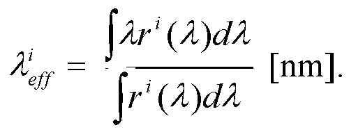 (4)
(4) Likewise, the effective solar flux at 1 AU for filter i is defined as
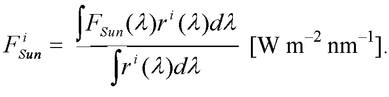 (5)
(5) We use the MODTRAN[4] zero-air-mass solar flux FSun(λ) at 1 AU in [W m�2 nm�1], resampled to the VIR spectrometer resolution. The signal Si (in DN/sec) observed through filter i can be converted to (spectral) radiance Ii by division through the responsivity Ri:
The clear filter responsivity is calculated as
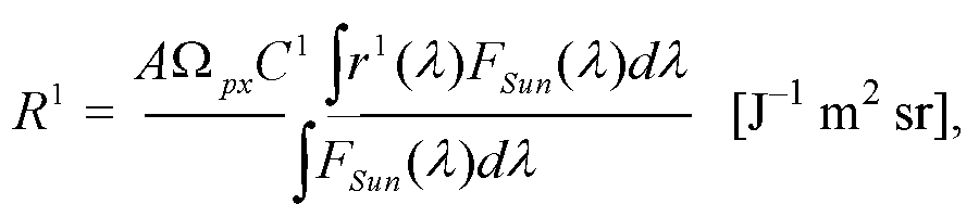 (7)
(7) in which A = 3.41x10�4 [m] is the FC aperture area [6], and Ωpx = 8.66x10�9 [sr] is the solid angle of a single pixel. For the color filters (i = 2-8), the responsivity is calculated in a slightly different way:
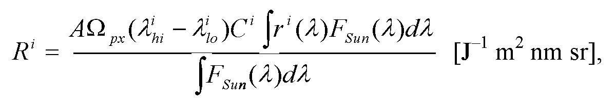 (8)
(8) in which λilo and λihi are the lower and upper boundary of the filter transmission FWHM (Table 2). The correction factors Ci follow from a comparison of predictions from the ground calibration with results from in-flight observations of standard stars (see below). Note that these responsivities are based on the assumption that the target has a solar spectrum.
If the target is a reflecting body like Vesta, radiance can be converted into reflectance, or "I/F", using the effective solar flux values in Table 2. For the color filters (i = 2-8):
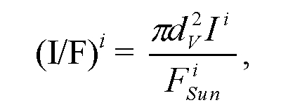 (9)
(9) where dV is the distance of Vesta to the Sun in AU at the time of the observation.
During the ICO Performance and Calibration blocks several photometric standard stars were observed to verify the lab responsivity. Vega (spectral type A0V) was observed by both cameras during Performance. In the Calibration block FC1 and FC2 observed 73 Ceti (B9III) and 42 Pegasi (B8V), respectively. Stellar spectra in absolute flux units were retrieved from the European Southern Observatory web site [5]. Some observations were pointed, others were acquired with the spacecraft slowly slewing such that the star point spread function (PSF) would cover different parts of the CCD. The star images were corrected for bias and dark current, and the result was divided by a flat field. We composed flat fields by dividing the fields shown in Figure 1 by third-order polynomial surface fits, the result being artificially flattened flat fields. The observed stellar flux was calculated as the total charge of a 15x15 pixel sized box centered on the star (determined from a 2D Gaussian fit), corrected for background intensity (estimated as the median value of a 100x100 pixel sized area around the star). The box dimensions are large compared to the small FWHM of the PSF (1.0-1.6 pixels, depending on filter [1]), but were chosen to include the broad wings. The expected flux for each filter was obtained by integrating the product of the stellar spectrum with the responsivity curves displayed in Figure 8.
We find the observed flux to depend strongly on the position of the center of the PSF with respect to the center of the pixel, being highest when both coincide. It is most sensitive to the distance to the center in the horizontal direction (example in Figure 9) due to the presence of the anti-blooming gates on the CCD, which run top-to-bottom. These, and other structures that run horizontally across the CCD, result in a low fill factor and quantum efficiency (around 0.2). To enable a comparison with the lab calibration we need to take the average of a representative sample of observations through each filter. Such a sample is available for Vega (n ~10), where 42 Peg and 73Cet were observed only twice per filter.
Figure 10 shows that the observed stellar flux is significantly higher than that expected from the lab calibration. The large spread in the data is the result of the low CCD fill factor. The results for both cameras are very similar, except for the smaller standard deviations of the FC2 Vega data, which indicates that FC1 pointing was more stable during exposure (unstable pointing would essentially create similar averages over the pixel). The average ratio of observed and expected flux in the clear filter (F1) is 1.11 for both cameras. It is around 1.1 for all color filters except F8, which has a ratio of 1.3-1.5. The F4 and F5 ratios are consistently higher (i.e. for both models) for 73 Cet and 42Peg than for Vega. The spectral type of 73 Cet is virtually identical to that of 42Peg but significantly different from that of Vega in exactly the F4 and F5 wavelength range. This suggests the problem lies with the standard star spectra, and may be due to a complex of water absorption bands in the 900-1000 nm wavelength range that affect standard star observations through Earth's atmosphere. Note that broad band filter F1 would be relatively insensitive to this. These results indicate that (1) the responsivity of both cameras is the same, and (2) that it is equal to that determined in the laboratory multiplied by a factor ~1.1 for all color filters except F8. The calibration pipeline is implemented based on these assumptions, using the following correction factors
for both cameras (Eqs. 7 and 8). The factor for F1 is chosen slightly higher than those of F2-F7 because the factor for F8 is so much higher.
The ICO standard stars are biased towards the early spectral type, ideal for accurately calibrating filters on the blue side of the spectrum (F2 and F8). The flux of solar analog stars is more balanced over the FC wavelength range. We verified the responsivities in Table 2 by fitting a solar spectrum to measurements of solar analog 51 Pegasi (G5V) acquired in the ICO Calibration block. Because 51 Peg is so much fainter than Vega the required exposure times are much longer. Spacecraft movement during a long exposure tends to move the PSF across the pixel, resulting in an averaged signal, as if the star were extended instead of a point source. Consequently, the flux reconstructed from individual images of 51 Peg do not show the large variability found for images of Vega. Figure 11 (left) shows the good agreement with the solar spectrum. Even though the S/N is very low for F8, it too agrees very well, confirming the validity of the 1.4 correction factor used to calculate the F8 responsivity. At Mars (MGA) we had the chance to verify the validity of the F5 responsivity in Table 2. Figure 11 (right) shows how the average intensity of light reflected off a small (100x100 pixels), uniform area on the surface in the F5 image is just below that expected for bright red soil, which is widespread on the Martian northern plains.
The conversion from DN to intensity by means of a single responsivity value is only valid if the CCD response is linear with exposure time. A series of flat field exposures with stepwise increasing exposure time was acquired on 12 Aug 2005 with the FC2. The CCD temperature was constant within one degree around 233K. The mean charge rate of a 100x100 pixel sized block in the lower left corner, which contains no insensitive pixels, is roughly constant up to a median charge of 7000 DN (Figure 12). Beyond this, the charge rate drops to a 2% lower value near full well (16383 DN). No such extensive data set is available for FC1, but an analysis of a more restricted set of flat fields (acquired on 24 Feb 2006) shows consistent behavior withthat of FC2 (Figure 12). The drop in charge rate towards full well is smaller than that reported earlier [8].
'Bad' pixels are pixels that fail to sense light levels correctly or have an unpredictable but high dark current. This encompasses both "dead pixels" which do not provide any signal at all, and "hot pixels" as extreme or unpredictable cases of warm pixels. Some have tentatively been identified for FC1 [3], and we are in the process of mapping them for FC2. Bad pixels will be removed by replacing their value with average of surrounding pixels.
We determined the degree of geometric image distortion by analyzing images from the ICO Performance and Calibration blocks, which had the FC point at star field targets. We follow the description by Heikkilä and Silvén (1997)[6]. Let (xu, yu) be the (undistorted) CCD coordinates of a star (measured in [mm] from the center of the CCD) that would result from an idealized pinhole camera projection. Then
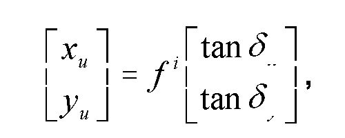 (10)
(10) with f i the focal length for filter i in [mm], and d the angle at which the star is observed in the sky (in radians). The true (distorted) horizontal CCD coordinates (xd, yd) in [mm] are different due to radial and tangential distortion:
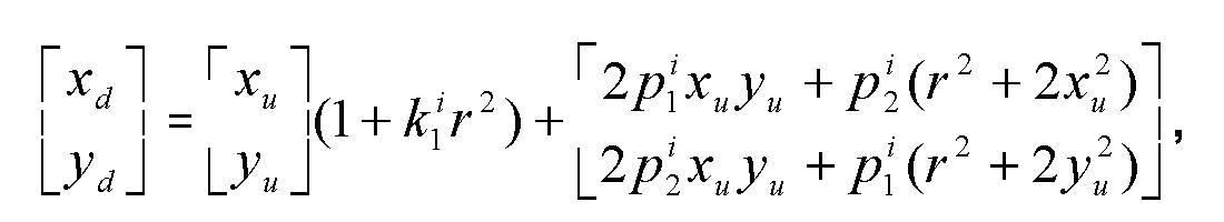 (11)
(11) with r2 = xu2 + yu2. The distance coordinates (xd, yd) are translated into pixel coordinates (u, v) as follows:
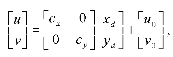 (12)
(12) with coefficients (cx, cy) in units of [mm�1], and (u0, v0) = (511.5, 511.5) the coordinates of the center of the CCD in pixels. The coefficients (cx, cy) map millimeters to pixels in the focal plane x- and y-directions, and are identical to the inverse of the pixel size. If cx = cy the CCD pixels are square. We know that the physical pixels are square to one part in a thousand (the manufacturer lists the CCD dimensions as 14.34x14.34 [mm2]), but we can determine the focal length with a higher accuracy than that. We therefore assume that the pixel size is 14.000 [µm] in the y-direction, and estimate cy / cx from the data. Thus, we use a 5‑parameter model for image distortion in each filter i: the focal length f i, the radial distortion parameter ki1, the tangential distortion parameters pi1 and pi2, and the ratio cy / cx, given cx = 71.409 [mm�1]. We verified that the optical axis coincides with the center of the image.
The star field around 20 Cepheus was imaged during the ICO Performance (December 2007) and DC041 (July 2010) campaigns. For 149 stars in this field we retrieved the International Celestial Reference System (ICRS) sky coordinates (in R.A. and Dec.) from the SIMBAD database [7], and fitted our model to their observed positions, estimated through a 2D Gaussian fit to the stellar brightness profiles. We find the FC focal length to be around 150.1 [mm], the exact value depending on filter (Table 3 and Figure 13). Given the CCD dimensions of 14.34x14.34 [mm2], this results in a FOV of approximately 5.47° squared; the IFOV values for each filter are listed in Table 3. Including radial distortion typically improved the fit to the star positions by 10-15%. Only the first order radial distortion parameter (k1) is significantly different from zero. For all filters k1 is found to be larger than zero, which implies that the FC suffers from slight pincushion distortion, amounting to half a pixel in the image corners. Including tangential distortion improved the fit by a further 5%, but the p1 and p2 parameters are badly constrained, and essentially were found to vary from image to image. The final fit results in Table 3 were obtained by assuming zero tangential distortion. The degree of radial distortion depends on wavelength, a phenomenon known as lateral chromatic aberration (Figure 13). We adopt the k1 values that result from a linear fit to the data (Table 3). In addition, we find the CCD pixels to be slightly larger in the horizontal (x) than the vertical (y) direction, with cy / cx = 1.00063+/-0.00003 (averaged over all filters). The final residuals of the fit of the model in Eqs. 10-12 and the parameters in Table 3 are typically around 0.1 pixel, and smaller than 0.3 pixel for almost all stars. For example, the RMS in the x- and y-direction are 0.091 and 0.110 pixels for a 15 [s] F1 exposure during DC041 (n = 87). The residuals may partly result from the inability of the Gaussian fit algorithm to find the true center of the stellar brightness profile due to the low pixel fill factor. We verified that the focal lengths and distortion parameters did not change in the period between ICO Performance and DC041. Both cameras appear to be very similar with respect to their geometric distortion characteristics.
The focal lengths were retrieved with high accuracy, and the differences between the filters can play a dominant role in the geometric distortion. Furthermore, the CCD pixels are significantly non-square, i.e. rectangular. For example, images corrected for geometric distortion acquired in filters F3 and F8 differ in size by about one pixel in the image corners. Not correcting color composites of the sky for differences in focal length leads to noticeable color separation for stars. Radial (pincushion) distortion is significant, and k1 parameters were retrieved with reasonable accuracy for each filter. Tangential distortion is insignificant, and consequently the p1 and p2 parameters could not be estimated reliably.
Table 1. Integrating sphere images averaged for flat field construction. FC1 flat fields were acquired on 24 Feb 2006 (TCCD ~ 230 [K]), FC2 flat fields on 12 Aug 2005 (TCCD ~ 233 [K]). The time stamp for FC1 image 30044 is 15h25m16s, that of FC2 image 26169 is 01h27m48s.
   ===========================================================================
   Model      Filter      Image #                                       n
   ===========================================================================
    FC1        F1          30044-30046, 30053-30055                     6
               F2          30060-30062, 30069, 30070, 30072             6
               F3          30076-30078, 30085-30087                     6
               F4          30092-30094, 30101-30103                     6
               F5          30108-30110, 30117-30119                     6
               F6          30124-30126, 30133-30135                     6
               F7          30140-30142, 30149-30151                     6
               F8          30178-30182                                  5
   ----------------------------------------------------------------------------
    FC2        F1          26169-26174, 26176-26178                     9
               F2          26484-26488, 26490, 26492, 26493             8
               F3          26506-26515                                 10
               F4          26528-26537                                 10
               F5          26539-26548                                 10
               F6          26517-26526                                  9
               F7          26495-26498, 26500-26504                     9
               F8          26475-26482                                  8
   ===========================================================================
Table 2. Filter characteristics, absolute responsivity, and effective solar flux for both cameras and all filters. lcen and leff are the filter band center and effective wavelength, respectively, in [nm]. The radiance is obtained by dividing the pixel signal (in DN / sec) by R. The result of this division has units as indicated in the rightmost column. FSun is the effective solar flux in [W m�2 nm�1] at 1 AU (see text).
| Filter | λcen | FWHM | λeff | FSun | R | Radiance unit |
|---|---|---|---|---|---|---|
| F1 | 735 | 371 | 732 | 1.365 | 5.12x10⁴ | [W m�2 sr�1] |
| F2 | 548 | 43 | 555 | 1.863 | 1.84x10⁶ | [W m�2 nm�1 sr�1] |
| F3 | 749 | 44 | 749 | 1.274 | 3.76x10⁶ | [W m�2 nm�1 sr�1] |
| F4 | 918 | 45 | 917 | 0.865 | 1.78x10⁶ | [W m�2 nm�1 sr�1] |
| F5 | 978 | 85 | 965 | 0.785 | 1.74x10⁶ | [W m�2 nm�1 sr�1] |
| F6 | 829 | 36 | 829 | 1.058 | 2.30x10⁶ | [W m�2 nm�1 sr�1] |
| F7 | 650 | 42 | 653 | 1.572 | 3.06x10⁶ | [W m�2 nm�1 sr�1] |
| F8 | 428 | 40 | 438 | 1/843 | 2.05x10⁵ | [W m�2 nm�1 sr�1] |
Table 3. Geometric distortion characteristics of each filter (focal length f, radial distortion parameter k1, and the IFOV), found by fitting ~100 star positions in ICO Performance (FC1 and FC2) and DC041 (FC2 only) images of the field around 20 Cep (p1 = p2 = 0). Two images were acquired per filter, so n = 2 for FC1 and n = 4 for FC2. The numbers in brackets in the k1 column are predictions based on a linear fit to the measurements (Figure 13). The focal length values are based on a pixel size in the x- direction of 14.004 µm. IFOV is in radians for the x- and y-direction.
   ================================================================================
   Model   Filter          f                 k1                         IFOV
                          [mm]              10�6[mm�2]                    10�5
   ================================================================================
   FC1       F1     150.074+/-0.004        7.6+/-0.1                9.3242x9.3184
   --------------------------------------------------------------------------------
   FC2       F1      150.074+/-0.006      8.4+/-0.4                 9.3242x9.3184
             F2      150.105+/-0.012      6.8+/-1.2 (6.7)           9.3223x9.3165
             F3      150.044+/-0.005      9.0+/-0.4 (8.4)           9.3261x9.3202
             F4      150.119+/-0.008      9.8+/-0.6 (10.0)          9.3215x9.3156
             F5      150.158+/-0.011      9.4+/-1.3 (10.3)          9.3190x9.3132
             F6      150.081+/-0.013      8.6+/-1.3 (9.2)           9.3238x9.3179
             F7      150.055+/-0.002      7.2+/-0.4 (7.6)           9.3254x9.3196
             F8      150.380+/-0.010      5.3+/-1.7 (5.6)           9.3053x9.2994
   ================================================================================
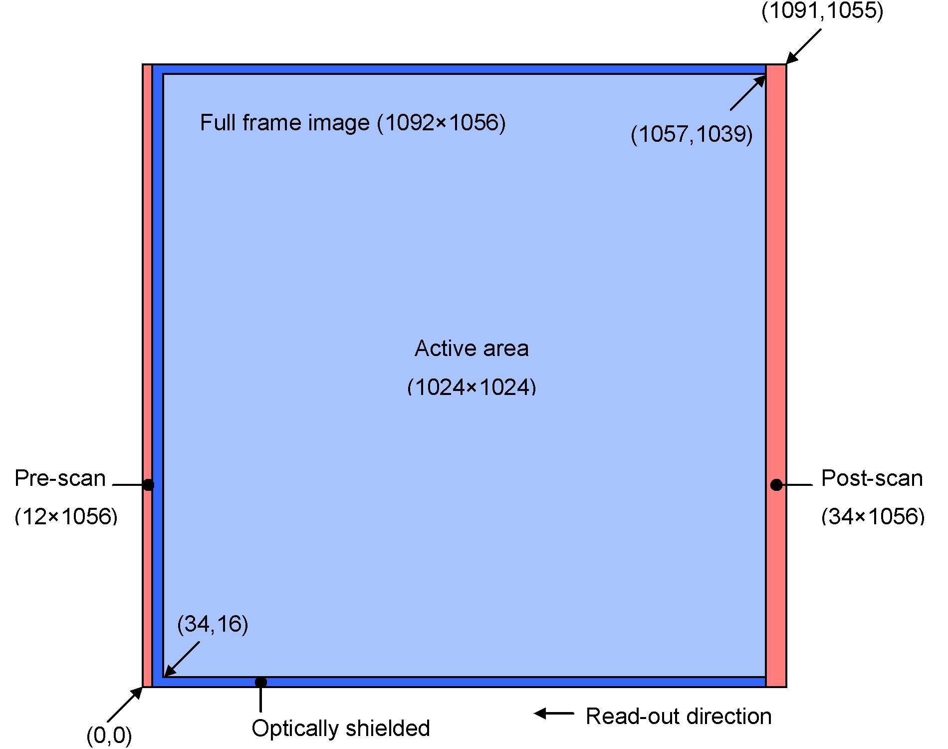
Figure 1. Layout of a full frame image (to scale). The active area is displayed in light blue, the optically shielded regions in dark blue, and the pre- and post-scan regions in red (note that these are not physically part of the CCD). Area size is indicated in (columns x rows). The coordinates of the pixels in the lower left and upper right corner of the full frame are (0,0) and (1091,1055), respectively. The coordinates of the pixels in the lower left and upper right corner of the active area are (34,16) and (1057,1039). When we consider the active area only, we refer to these pixels as having coordinates (0,0) and (1023,1023). The storage area is located below the area shown here. The horizontal (read-out) direction is referred to as the sample- or x-direction, the vertical direction is the line- or y-direction, consistent with the definitions in the SPICE kernels.
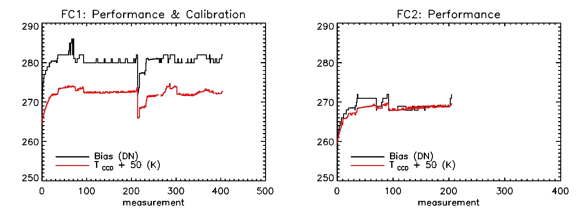
Figure 2. The bias of FC1 images acquired during the ICO Performance and Calibration blocks compared to the CCD temperature. Left: FC1, right: FC2.
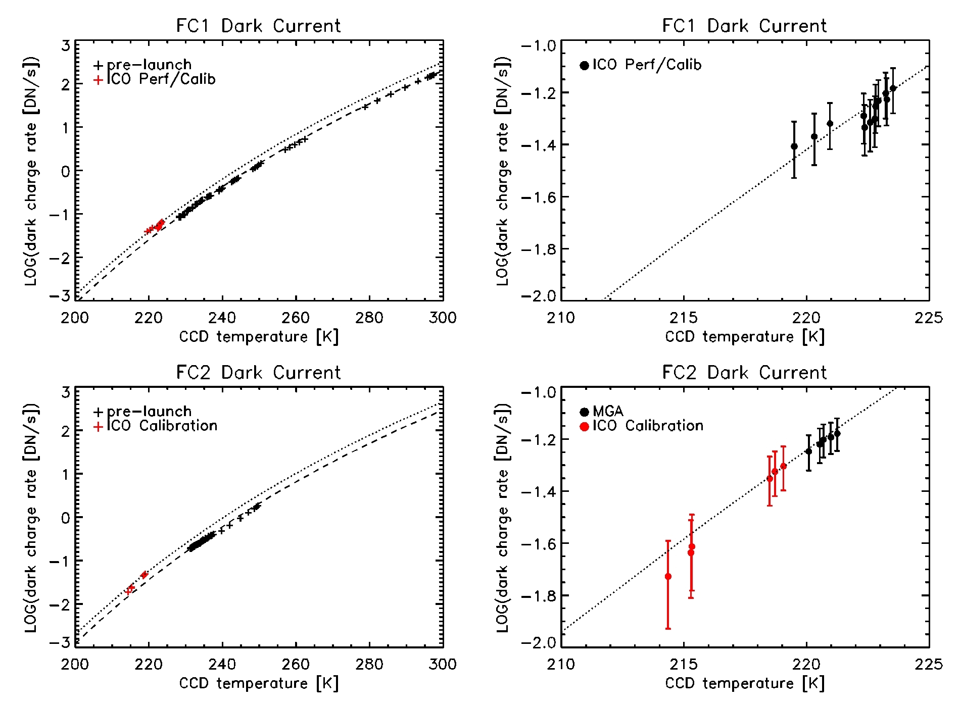
Figure 3. Pre- and post-launch dark current in [DN/sec] of a typical CCD pixel, calculated as the mean of row 1000. The post-launch data (ICO/MGA) represent 300 [s] exposures only. The lines are fits of the model in Eq. 1 through the pre- and post-launch data (dashed and dotted lines, respectively). Post-launch data are corrected for warm pixels and cosmic rays.
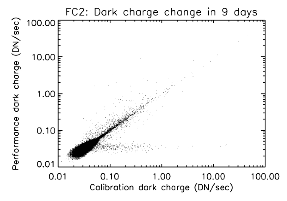
Figure 4. FC2 dark current evolution over the course of the 9 days from the ICO Performance to the Calibration blocks. New warm pixels are located in the horizontal branch at the bottom.
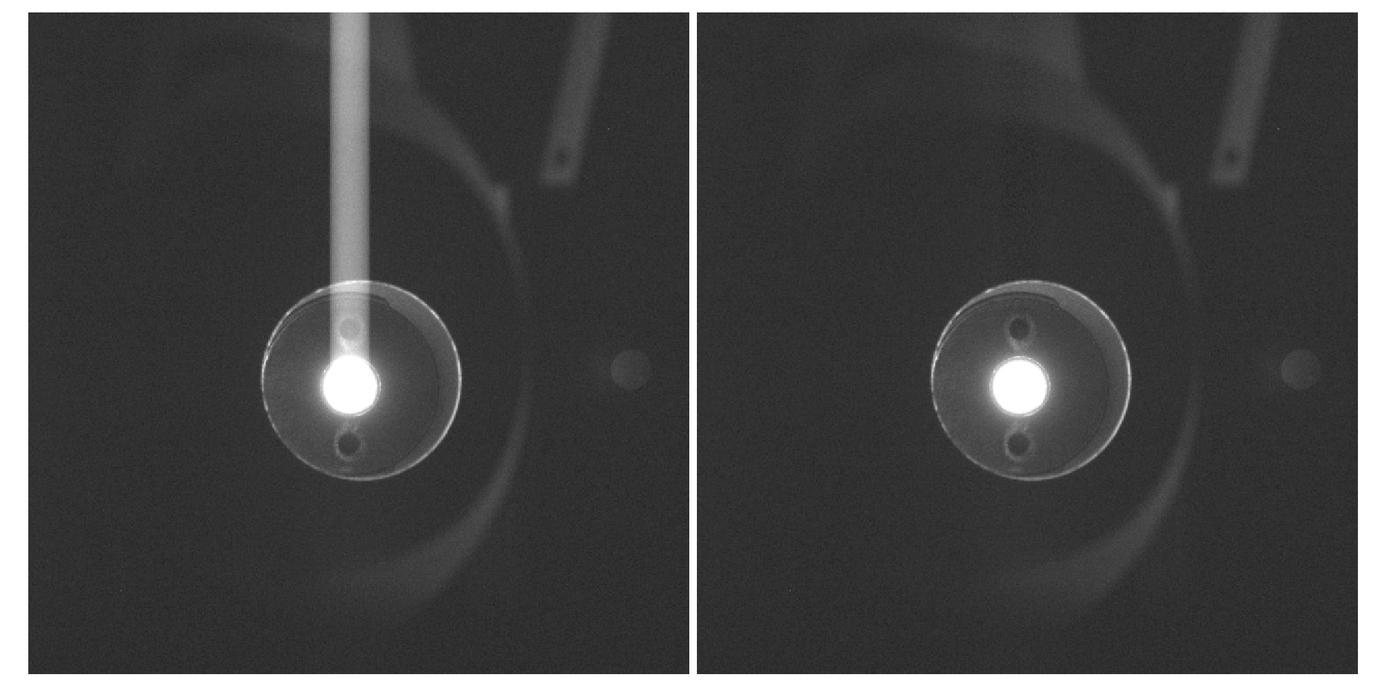
Figure 5. The de-smear algorithm in action. The FC1 observed an illuminated pinhole through a collimator through F1 (8 Mar 2006). Exposure time was 60 [ms]. Left: original image (average of two). Right: image after de-smearing. The brightness is scaled identically in both, such that black and white are equivalent to �5 DN and 30 DN, respectively. The peak signal in the central spot was 13110 DN. Note that a weak ghost is visible at the right of each image.
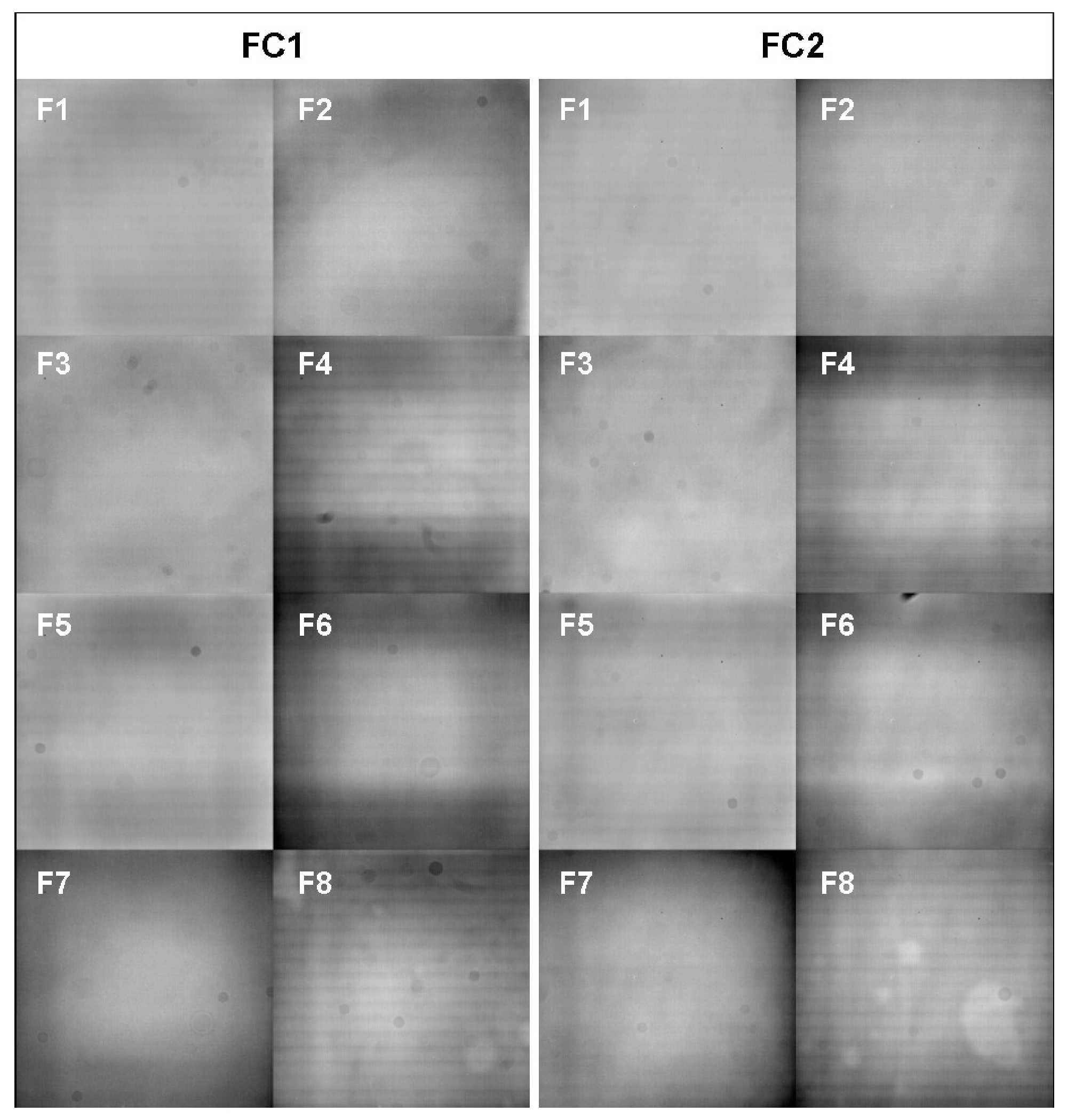
Figure 6. The normalized flat fields of FC1 (left) and FC2 (right). Brightness is scaled such that values <0.90 are displayed as black, and values >1.05 as white. A faint diagonal pattern is due to stray light associated with the experimental setup.
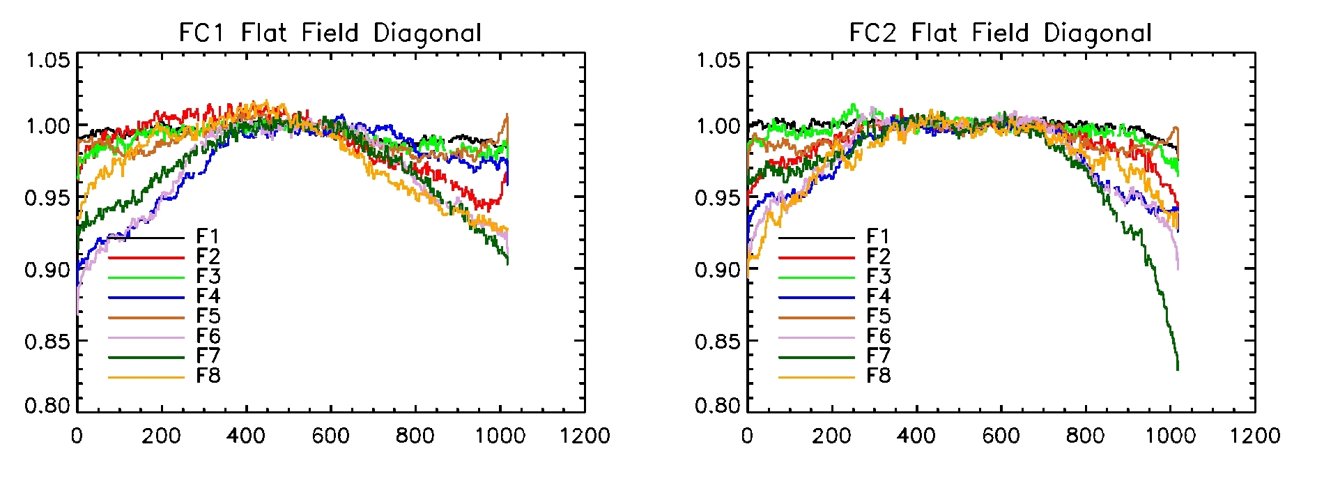
Figure 7. Diagonal profiles through the flat fields in Figure 6, running from pixel [0,0] to [1023,1023]. The profiles have been subjected to a 7-pixel wide median filter.
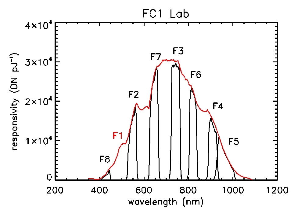
Figure 8. The FC1 absolute responsivity for the different filters as determined from the lab calibration.
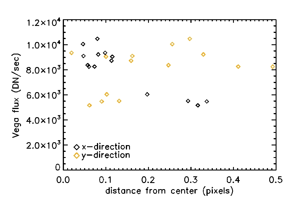
Figure 9. The measured flux of a point source (in this case Vega observed by FC1 through F7) depends strongly on the position of the PSF on the pixel, especially in x-direction because of the presence of anti-blooming gates. The x-axis denotes the distance of the center of the PSF to the center of a pixel, as determined by a 2D Gaussian fit.
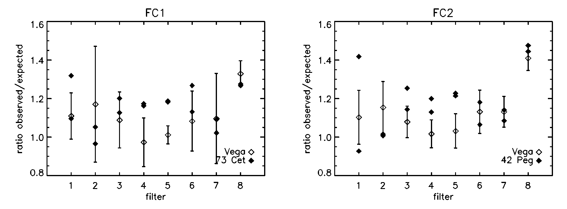
Figure 10. The flux of three photometric standard stars observed by FC1 (left) and FC2 (right) for all filters compared to that expected if the lab calibration in Figure 8 were correct. The Vega data are the mean and standard deviation of ~10 observations. The 73Cet and 42Peg data are two single observations per filter.
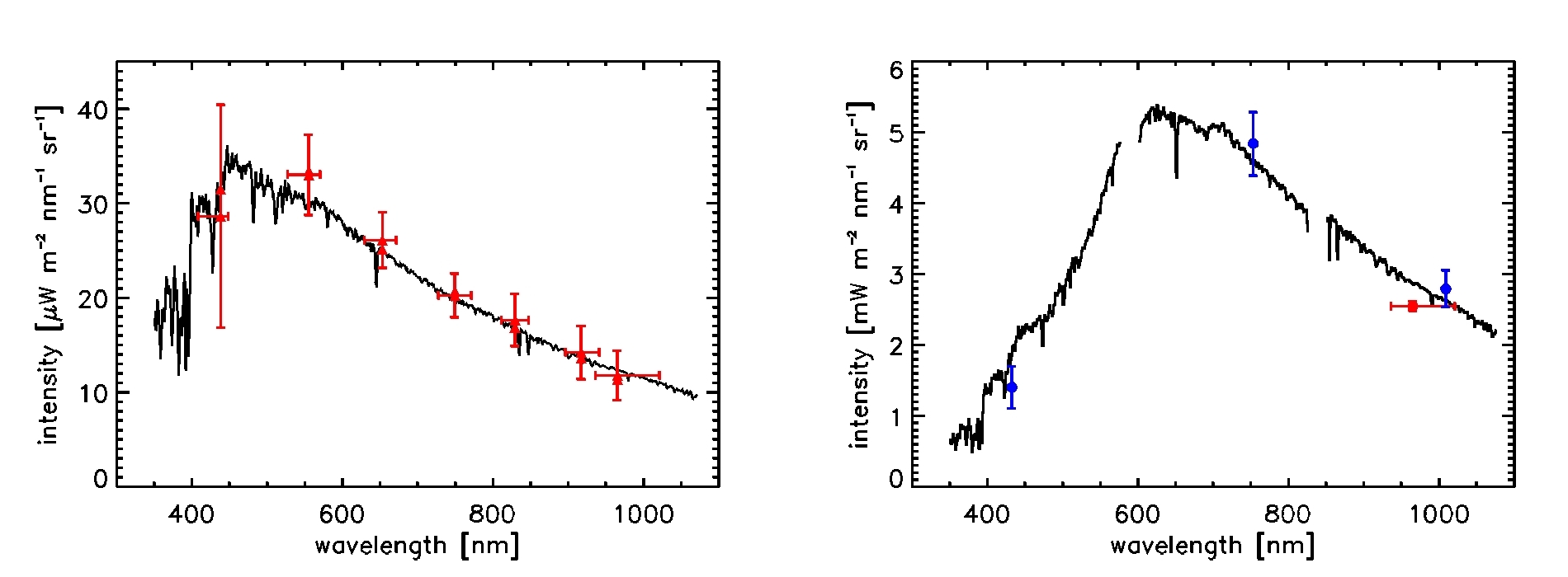
Figure 11. Verification of the responsivities in Table 2. Left: The solar spectrum (black) fitted to the intensity of solar analog 51 Peg (red triangles), observed during the ICO Calibration block. The intensity was integrated over a 15x15 pixel block surrounding the star. There were two observations in each filter; for clarity, error bars are shown for only one. Right: Reconstructed intensity coming from the Martian surface for F5 image 1010, acquired during MGA. The plot compares the reconstructed intensity (red bullet; calculated with the F5 responsivity in Table 2) to that expected for the ubiquitous bright red soil (black line). The expected spectrum was calculated by scaling the Mars geometric albedo to bright soil BRDF measurements by the Spirit rover for the FC observation phase angle (blue bullets; from Johnson et al. [2006] JGR 111, E02S14).
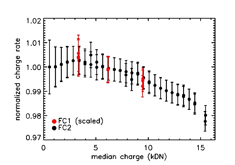
Figure 12. Investigation of CCD linearity. Shown are the mean FC1 and FC2 charge rates in a 100x100 pixel block in the lower left corner as a function of median charge in lab flat field images (FC1: 24 Feb 2006; FC2: 12 Aug 2005). The FC2 charge rate is normalized to that associated with the lowest median charge. The FC1 charge rates were higher, but scaled to match the FC2 series. Some scatter in the data is due to uncertainties in exposure time.
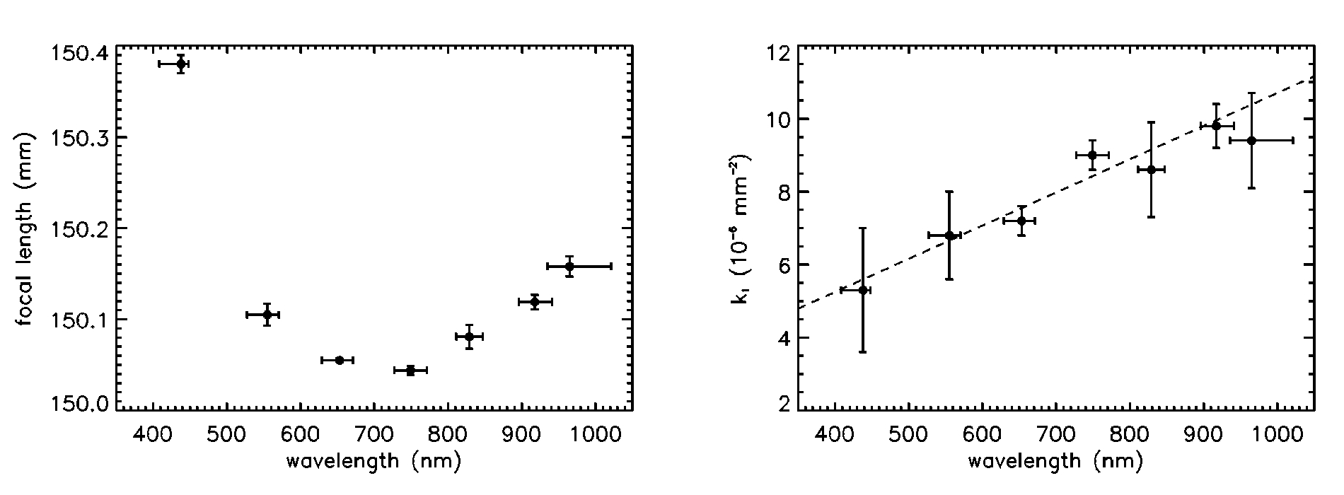
Figure 13. FC2 geometric distortion characteristics. Left: Focal length as a function of wavelength. Right: The radial distortion parameter k1 depends on wavelength (lateral chromatic aberration). The dashed line is a linear fit to the data.
The calibration pipeline has been implemented as a stand-alone executable named Calliope that runs on an MPS server. The executable implements a fixed architecture of the algorithm, but the parameters to the algorithm are supplied by a configuration file that is distributed with the executable. The algorithm needs a number of reference images to calibrate the science images. These are also distributed with the executable, and their location is specified in the configuration file.
The executable has been implemented in C++ and its architecture is intended to mirror that of the algorithm. In essence, it is composed of a set of atomic processing blocks (i.e.: bias subtraction, dark current removal) linked together according to the algorithm. Each atomic block receives an image in a certain state, processes it, and forwards the updated image to the next block. The concept is simple, but in order to make it work the collection of atomic blocks has been expanded with other blocks that are not related to the calculations. Examples of this are filters (that forward the image through one of two paths depending on a condition), folders (that take a folder name and forward all the images in the folder to the next block) and savers (that write images to file). A number of savers can be activated in the configuration file to save intermediate images in the calibration pipeline.
The current pipeline implementation is shown in Figure 14. The processing chain starts with a folder that reads all the PDS files in a given folder, examines the attached PDS label to ensure that these are indeed FC images, and forwards them to the next step one-by-one. Files that are not FC images are discarded. The next step is to separate the different types of images depending on the acquisition mode. Serial images, test patterns, and storage readouts need not be calibrated further, so they are simply dropped. Dark images, calibration lamp images (which are tagged as 'flat fields' in the PDS header), and normal (regular) images are passed on. Images can either be full frame (1092x1056 pixels), or have the active area (1024x1024 pixels) and extra regions attached as separate frames. Images that are composed of several sub-images or 'windows', have a separate 'summary frame' attached. This summary frame is reconstructed (on ground) to show the relative location and orientation of the (smaller) windows within the full frame, with non-window pixels set to zero. At this point the summary frame is dropped, and the calibration is applied only to the windows. Note that at the end of the calibration pipeline the summary frame is reconstructed from the calibrated windows.
The next step is to transform the 16-bit integer image (active area) into 32-bit floating point format (in case the frame is not in floating point format already). At this point, if the image came as a single 1092x1056 frame, the pipeline splits it into one image frame and the extra regions. Now the calibration algorithm proper starts with the removal of the electronic bias. The bias is computed as the floating point average of the pre-scan frame (§2.1). If the image does not contains the pre-scan frame the pipeline stops processing, reports the error, and continues with the next image. The bias removal is applied to all image frames, including the pre-scan frame that will then have an average of zero. The bias-corrected images are then filtered depending on type of acquisition. Dark frames, typically used for dark current characterization, do not require further processing. Regular and calibration lamp images are transferred to the next block. If FC2 is found to suffer from extra charge (§2.2) then the next block is extra charge removal (not yet implemented), otherwise it is dark current removal.
As described in §2.3, the dark current in a given pixel is a function of the CCD temperature and the pixel properties. The correction is done by subtracting a dark image calculated from a reference dark image and the exposure time and CCD temperature. As before, if the reference dark image cannot be located, the pipeline notifies the error and stops processing. At his stage the image is corrected for smear resulting from the fast transfer into the storage region (§2.4).
Next comes flat fielding, the compensation for optical non-uniformities (e.g. dust specks on the filters). This is done by dividing the image by a normalized flat field (§2.5). There is a separate flat field for each filter and camera, so the configuration file has to specify 16 images. Once more, processing stops if a flat field cannot be found.
At this point, there is a separation into regular and calibration lamp images. The latter are divided by the effective illumination time, which is not strictly equal to the exposure time [8]. Regular images are divided by the exposure time, and radiometrically corrected to yield intensity in physical units (§2.6). The last step in the calibration process is geometric correction (§2.8), but there are no plans to implement this in the pipeline.
Now there are only three steps left. The first one is the disposal of the additional image frames (which are not illuminated and may have been used for calibration purposes). The second one is the re-generation of a summary frame in case the image consists of several windows. The final step is writing the calibrated image to file with the proper name and format.
The calibration pipeline configuration file is an XML file that stores the configuration parameters. The XML format allows for easy inspection and modification, and the file can be easily put under code configuration control. Its structure is based on hierarchical periods of time. The outermost (top level) object is a time period defined to include the full Dawn mission. Other time periods can be defined as 'children', recursively inside this period. Examples are mission phases, observation sessions, and observation stations. Child time periods do not overlap those of their siblings (to avoid decision problems), and are fully enclosed by those of their parents.
The configuration parameters are defined by pairs of keyword names and values. For each period of time, regardless of its depth in the structure, any number of keyword values can be defined. During execution, the pipeline reads from the header of an image when it was acquired, and then asks the configuration file what are the applicable keyword values for that point in time. If a keyword is defined in more than one level, the value on the deepest level is used. For instance, a general reference dark image can be defined for the full mission, while a specific reference dark image is defined for a specific phase of Vesta observations. All images taken in this phase will be calibrated with the specific dark image.
The configuration file defines for the period of time where each image is acquired the following values and files:
   ===========================================================================
   Value name     Type    Scope                   Definition
   FCx_Fy_Flat    Image   Per camera and filter   Reference flat field
   FCx_Fy_Rad     Value   Per camera and filter   Radiometric calibration coefficient
   FCx_Dark       Image   Per camera              Reference dark current
   Save_xx        Value   Global                  Switches for the savers
   Image_Folder   Value   Global                  Location of the above-mentioned files
   ===========================================================================
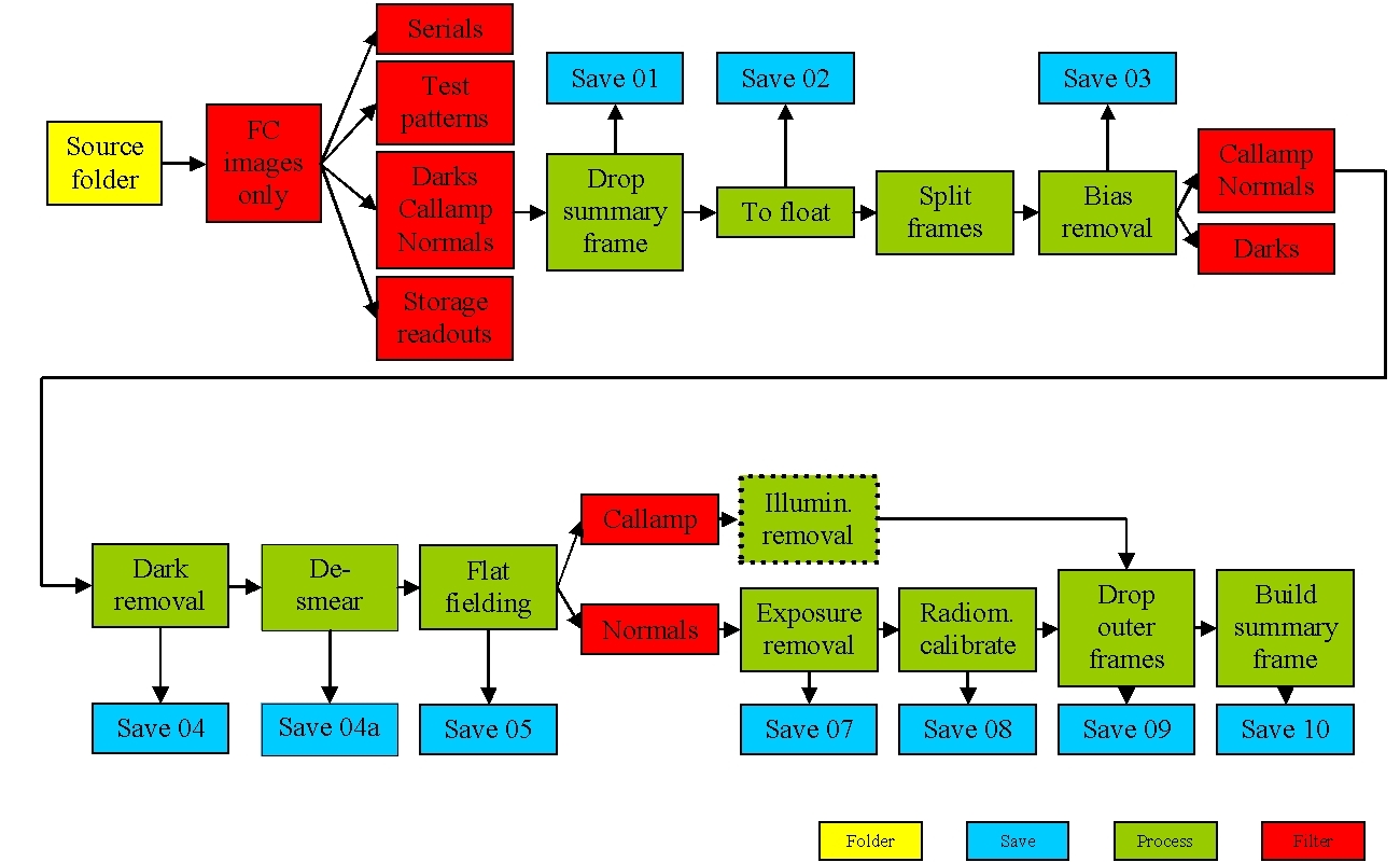
Figure 14. Flow chart for the calibration pipeline algorithm. 'Callamp' is an image of the inside of the camera cover illuminated by the internal calibration lamp (labeled 'flat field' in the PDS image header).
[1] The absence of a shutter means that the CCD is continuously exposed to light if Vesta is in the field of view and the door is open. The time between the start of an exposure and the previous read-out of the CCD is the "pre-exposure" time.
[2] Hawkins et al. (2009) In-flight Performance of MESSENGER's Mercury Dual Imaging System. Proc. of SPIE Vol. 7441, p. 74410Z
[3] Sierks et al. (2011) The Dawn Framing Camera. Space Sci. Rev.
[4] http://rredc.nrel.gov/solar/spectra/am0/modtran.html
[5] http://www.eso.org/sci/observing/tools/standards/spectra/
[6] Heikkilä and Silvén (1997) A Four-step Camera Calibration Procedure with Implicit Image Correction. IEEE Computer Society Conference on Computer Vision and Pattern Recognition (CVPR'97), San Juan, Puerto Rico, p. 1106-1112.
[7] http://simbad.u-strasbg.fr/simbad/
[8] The calibration time can be switched on before or after the beginning of the exposure time and can be switched off before or after the end of the exposure. Therefore the effective illumination time is min(end of exposure, end of illumination) � max (start of exposure, start of illumination)